Estimation of Mean Fixed Frequency Biases: the significance of BFO Channels

Geoff Hyman and Barry Martin
2015 March 19

(Report prepared in 2014 December)

A downloadable PDF of this report (627 kB) is available here.

Background
The focus of this report is the estimation of mean fixed frequency biases (FFBs), for applications to MH370 flight path analysis. This report investigates the extent to which the mean frequency bias is contingent on the number and type of channel associated with burst frequency offsets (BFOs). The approach adopted will be primarily via descriptive statistics; but a degree of hypothesis testing will be unavoidable. It is found that certain combinations of both channel type and number are significant covariates for the mean FFB, meriting consideration in improved modelling of MH370 flight paths. While investigation of the causes of factors of this kind are outside the scope of this paper, additional evidence on causation would be of interest, particularly if it can assist the air accident investigation.

This report represents a continuation of our analysis conducted in recent months, which was earlier restricted to conditions when MH370 was on the ground. The introduction of channel-specific biases has been identified and wider validation of their values is warranted. The current report includes BFO data for the early cruise phase of the flight. The sample size is increased from 131 ground observations to 263 total observations, which effectively doubles the sample size. Whilst the cruise data is somewhat more variable than the ground data, this increase in the sample size is sufficient to provide narrower confidence limits to our estimates.

One of the interesting findings here is that a simple split by channel type (R and T) is not the most effective way of identifying the inter-channel differences. A combination of channel type with channel number is needed for a more effective BFO analysis and in the assessment of competing flight path models.

Introduction
We estimate mean FFBs using ground and early-cruise BFO data, and the PAR5 satellite model (Reference [1]; see also this post).

The sample values of the FFB terms were calculated using [2]:

The FFBs are segmented by channel number (4, 8, 10, 11, and 12) and type (R, T). In the current data set channel 8 is the only channel number that appears as both type R and type T. Figure 1 shows the resulting FFBs against time (UTC) during the ground and early-cruise phases, based on the PAR5 satellite positions and velocities [1] and a model for the aeroplane position and velocity.

Figure 1: FFB variation over time by channel

Inspection of Figure 1 suggests that only three FFB values (for blue channels R4 and R11) exceed the lowest value for the other channels (151 Hz). This is good prima facie evidence of channels R4 and R11 differing from the others. This topic will be subject to statistical testing, as discussed below.

Table 1 shows, for each combination of channel number and type, the mean FFB, the standard deviation of the FFB, and the standard error of the estimated mean (the standard deviation divided by the square root of the count).

 Table 1: Initial FFB Descriptive Statistics by Channel

Stage 1 Tests
We now turn to an issue requiring some basic testing of hypotheses. The first question to be addressed will be: How do estimated FFB means for the BFOs associated with R4 and R11 differ from each other, and is this difference statistically significant? From the numbers given in Table 1 we would clearly expect to obtain a negative result. We will however proceed, for the purpose of illustrating the tests. We apply both a non-parametric and a parametric test. The non-parametric is the Mann-Whitney U-test [3], [4] and the parametric is the Welch-Aspin test [5]. The Welch-Aspin test accommodates both unequal group sizes and unequal group variances. The Mann-Whitney test only requires information about rank and is distribution-free.

Both tests yield a test statistic that is a ratio of a measure of difference to a measure of its standard error. In both tests we will refer to this statistic as its Z-score. We may consider a Z-score in excess of 3, in both tests, to be significant. A Z-score in excess of 5 in both tests (the ‘five-sigma level’) is taken to be highly significant.

Table 2 contains the results for R4 versus R11. The non-parametric Z-score is 1.45 and the parametric score Z-score is 2.13. To reject the null hypothesis both scores were required to exceed 3, so we have not met this condition.

Table 2: Testing for differences between estimated means:
Channel R4 v channel R11

For the purpose of our current estimation task we treat R4 and R11 as equivalent channels. The distributions of the estimated means are presented stylistically below, as ‘spike plots’. These plots have been designed to give a visual indication of how well determined the FFB means are, given the input data being used for estimation. The x-axis denotes the FFB scale in Hz, with the peaks set at the estimated mean values. The width of each spike is two standard errors, one on each side of the estimated mean. The areas under the spikes are designed to be approximately equal, with the height of each spike set at the reciprocal of the corresponding standard error. Spike plots are given both before and after merging R4 with R11.

Figure 2: Spike plots by channel, before and after merging R4 with R11

The next test of interest is the statistical significance of the differences between the estimated means for the R4+R11 combination and the combinations of the other channels: T10+T12+R8+T8.

The results are given in Table 3. The non-parametric Z-score value is in excess of 7 and the parametric Z-score value exceeds 19. This is to be taken as a highly significant difference between the estimated FFB means for the R4+R11 combination and the combination of the remaining channels. The relative offset has a value of -3.9 Hz, i.e. the mean FFB for R4+R11 is nearly 4 Hz lower than the mean FFB for the other channels combined. The Z-score values for both tests exceeded the five-sigma threshold, leading to a strong rejection of the null hypothesis so that, in the absence of a true systematic difference, the reported results should typically appear no more than once in (at least) 3.5 million trials.

Table 3: Testing for differences between channel
R4+R11 vs all other channels combined

Table 4 provides the descriptive statistics for the resulting two-way split between channels, corresponding to the greatest two-way differentiation available from the data being used. While this may be incorporated in the analysis of flight paths, it is of interest to investigate whether the data would support a further level of discrimination.  

Table 4: FFB Descriptive Statistics after Stage 1. 

Now suppose that instead of splitting the channels in this way we had simply split them according to type (R, T). What would we have obtained? Table 3 would have been replaced by Table 5 (below).

Table 5: Testing for differences between R and T channels

It can be noted that the result of this test produces a significant result, but it is not highly significant (at the 5-sigma level). Further, the relative offset between the T- and R-channels is only 1.3 Hz. The standard deviation for the grouping of R-channels has increased substantially, resulting in wider confidence bands for the mean FFB. On the current data set, the R/T segmentation would be inferior to that given in Tables 3-5 and was not retained for the next stage in the analysis.

Stage 2 Tests
We now take a closer look at the time (UTC) profile of the FFBs for the four unmerged channels: T8, T10, T12 and R8.

From Table 1 it looks like T12 might have a slightly lower mean FFB than the three remaining groups, T8, T10 and R8. If we were to merge the latter three we would arrive at the grouping of channels depicted in Figure 3.

Figure 3: Spike plots by channel combination,
after merging R8, T8 and T10.

How does the estimated mean FFB for T12 differ from the estimated mean FFB for the R8+T8+T10 combination? The results of the two tests are given in Table 6. The Z-score values for both tests exceeded the three-sigma threshold, indicating that, in the absence of a systematic difference, the null hypothesis would be incorrectly rejected with an (estimated) expected frequency of less than one in 300. The result is considered significant, but not highly significant. The relative offset is 0.54 Hz, so that the mean FFB for T12 is approximately one half of a hertz (0.5 Hz) smaller than the others.

Table 6: Testing for differences between mean FFBs for
channel T12 vs channel combination R8+T8+T10

The descriptive statistics for the resulting channel combinations are given Table 7.

Table 7: FFB Descriptive Statistics after Stage 2.

In the flight path analysis the principal statistics that are used are the means and standard deviations for the channel number and type associated with the BFO applicable to the phase of flight under investigation.  These statistics are depicted in Figure 4, illustrating the detailed distinctions obtained from both the Stage 1 and Stage 2 analyses.

Figure 4: FFB means and standard deviations for
identified channel groupings

Figure 4 shows how an all-channel mean of 153.86 Hz first becomes split into two groups, with a -3.9 Hz difference between R4 + R11 and the remaining channels. The remainder then are split into two further groups, with a -0.54 Hz difference between T12 and the other channels.

Discussion and Conclusion
The findings from the Stage 1 analysis appear to be particularly robust and support the broad findings of the ground-based analysis, at a high level of statistical significance. Alternative forms of Stage 1 segmentation, such as a simple split by channel type, did not provide the same level of discrimination. The results from the Stage 2 analysis are currently tentative, and the level of discrimination that it provides is modest.  Pending a deeper understanding of these issues, it is recommended that only the results from Stage 1 should be used in MH370 flight path analysis.

References

[1] Rydberg, H. (2014): PAR5 satellite vectors/ephemeris

[2] ATSB (2014): ATSB report June 2014 updated August

[3] Mann & Whitney U-test

[4] Mann & Whitney (1947) 

[5] Welch t-test

 

Calibration of the Mean BTO Constant

Geoff Hyman and Barry Martin
2015 March 19

(Report prepared in 2014 November)

A downloadable PDF of this report (542 kB) is available here.

 

Introduction and Summary

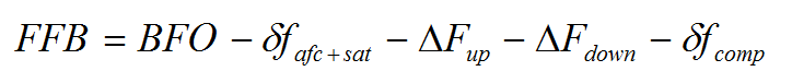
We seek to estimate the mean value of K in the BTO equation:

 

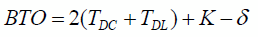
Here TDC refers to the time delay in the C-band (satellite to Perth) signal and TDL to the time delay in the L-band (aeroplane to satellite) signal.

Further details on the calculation of the individual observations may be obtained from Reference [1]. BTO data were available for two types of channel: R and T (Reference [2]). Their associated K values have different means and the offset δ is applied to all of the T-channel observations to allow them to be combined with R-channel observations which maximises the total sample which can be used for estimation. We adopt the convention of setting the offset δ to zero for R-channel observations. The values of K typically vary between observations, so that:

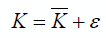
where K-bar is an unknown but constant mean value that we seek to estimate and ε is a residual. For the purposes of calibration the residuals are assumed to be randomly distributed with a mean of zero, have a constant variance, and to be uncorrelated. The value of K-bar is estimated by averaging the K values derived from a suitable sample. In a minor abuse of notation we will also use the symbol K-bar when reporting estimates of its true value, which is unknown.

The plan of this report is as follows. In section 1 preliminary estimates for the mean BTO constant are obtained, examining sensitivity to the magnitude of the T-channel offset and exploring the difference between estimates based on conditions when the aeroplane is stationary with a wider data set when the aeroplane was on the ground. Similar values for the BTO constant were obtained provided the appropriate offsets were re-estimated for the dataset being adopted.

In section 2 a comparison is conducted with estimates published by the ATSB in its June 2014 report. The estimates made there for the mean BTO constant appear to be consistent with our initial findings.

In section 3 some preliminary conclusions are drawn.

In section 4, a review of data from the T-channel is conducted. This resulted in the need to filter out T-channel observations occurring less than a certain critical time after the preceding ones. Consistent estimates for the BTO constant were obtained but with wider confidence limits. We also briefly review a limited data set that includes the climb and early cruise phase, leading to a refinement in the data reduction method.

In section 5 the impact of using a new set of satellite vectors is discussed.

In section 6 a comparison is made between estimates from the reduced data set and estimates based entirely on BTO data for the R-Channel.

In section 7 we revisit the comparison between ATSB’s June estimate for the BTO constant and our latest estimates, using improved satellite position data. The ATSB estimate is also consistent with our revised estimates. It is concluded that the odds were somewhat against ATSB obtaining a value that was as close as was found to our latest estimate, but that this is not a surprising result.

1 Preliminary Estimation

An ensemble of ADS-B logs from numerous feeders [3] provides independent evidence of the aeroplane position history prior to deviation from the flight planned route. The ADS-B position timestamps have an error of ±10 seconds which translates to an along-track error of ±2.4 km, equivalent to an uncertainty in the aircraft-satellite range of the same order, in turn leading to significant BTO prediction errors. For this reason the aerial data were not used in determining the BTO constant.

This issue does not apply when the aeroplane is on the ground because the aeroplane position is well-determined so calibration to ‘ground truth’ will be adopted. Estimation was conducted for periods when MH370 was (a) static; and also (b) still on the ground, but including observations made when the aeroplane was both static and moving.

i) The T-channel offset δ was initially assumed to be 5000 microseconds.

ii) The offset δ value  was also optimised to minimise the resulting standard error of the estimated value of K-bar over the combined data for both channels. The resulting offset value was 4979.8 microseconds from 76 data points when the aeroplane was static, and 4976.6 microseconds from 137 data points for the entire period when the aeroplane was on the ground. No outliers were identified at this stage (i.e. all observations in their respective clusters were used).

The estimates for the BTO constant K are given in Table 1 (units in microseconds) using the ATSBX satellite position model. This ATSBX  model adopts a linear interpolation for each of the three Cartesian position components for seven vectors given at five-minute intervals over the period 1600 to 1630 UTC in Reference [4] (Appendix G, Table 1).

Further details of the ATSBX model are given in Reference [5] (Vectors).

ATSBX	Offset δ : 4979.8 μsec		Offset δ : 5000.0 μsec
	Static	Ground (all)	Static	Ground (all)
K-bar	-495679.3	-495677.5	-495672.1	-495665.3
Standard deviation of K	31.7	26.8	33.1	29.1
Count	76	137	76	137
Standard error of K-bar	3.63	2.29	3.80	2.49

Table 1: Initial Estimates for BTO constant K (all in microseconds).
Source: [5] (Statistics). All figures in microseconds. 

In Table 1 above, and the later tables, the row labelled ‘Standard error of K-bar’ refers to the standard error of the estimate for the mean value of the distribution of the random variable K (cf. the preceding equation for K-bar: K-bar = K + ε). It is closely related to the standard deviation of K, and is calculated using:

Standard error of K-bar = Standard deviation of K / SQRT(Count)

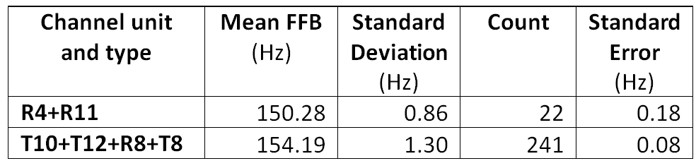
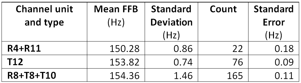
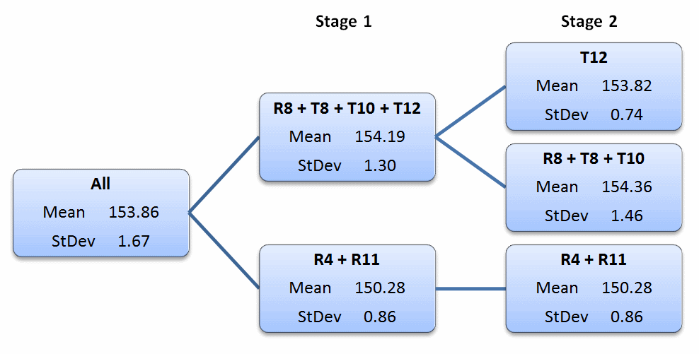
The full ground data set gives a lower standard deviation than the static set. This appears to be because of a greater preponderance of T-channel observations. The variability of K values from the T-channel appears to be much lower than from the R-channel so particular care needs to be taken when combining them in estimates of K-bar. The implications of this issue for estimating K-bar will be investigated in a later section.

When the T-channel offset is set to 5000 microseconds the mean K from the static and full ground data sets differ by 6.8 microseconds. If a standard error 2.49 microseconds (given in the last column of Table 1) was accepted then this difference would be statistically significant.  On the other hand, with the optimised T-channel offset, the mean K for the ground set differs by only 1.8 microseconds from the static mean K, which is not statistically significant. To investigate this further the statistics for a T-channel offset of 4976.6 microseconds, estimated from the full ground data, were tabulated in the last two columns of Table 2.

ATSBX	Static offset δ: 4979.8 μs		Ground offset δ: 4976.6 μs
	Static	Ground (all)	Static	Ground (all)
K-bar	-495679.3	-495677.5	-495680.5	-495679.5
Standard deviation of K	31.7	26.8	31.7	26.7
Count	76	137	76	137
Standard error of K-bar	3.63	2.29	3.64	2.28

Table 2: Implications of Static and Ground based offsets for the BTO constant. Source: [5] (Statistics). All figures in microseconds. 

Comparing the first and last columns we observe that the mean values for K (both underlined) differ by only 0.2 microseconds. It appears that similar mean K value are obtained irrespective of whether the static or full ground data are used, provided the appropriate T-channel offset is defined for the dataset being adopted, as indicated by the values that are underlined. On this basis the best candidate for the mean BTO constant, in integer microseconds, would be -495679 based on the static data, or -495680 based on the full ground data, with the appropriate T-channel offset in each case. For the purposes of risk analysis, it would be prudent to use the larger standard error of 3.63 obtained for the period when the aeroplane was static.

2 Comparison with ATSB June Estimates

In Reference [4] (Appendix G, Table 2) the ATSB give a mean BTO constant K of -495679(.3) microseconds. The decimal place given in brackets has been calculated from the values given in ATSB’s table and has been included to facilitate comparisons.

This is a fraction of a microsecond away from the value obtained by our analysis, and the difference is not statistically significant. Further examination of the ATSB data indicates that:
a) The ATSB estimate was based on only 17 data points, all from the R-channel;
b) The standard error of the ATSB estimate is 7.6 microseconds, substantially greater than the difference between ATSB’s estimate and those reported here; and
c) The median (50th percentile) of the ATSB values for K is -495661 microseconds, whereas the median for our estimates, from the full ground data, is -495680 so that these median evaluations differ by 19 microseconds.

It is concluded that the close similarity between ATSB’s estimate and ours is fortuitous. In a later section we will make a quantitative assessment of just how likely this might have been.

3 Preliminary Conclusions

Based on the current dataset, using the ATSBX satellite position model, the mean BTO constant is -495680 microseconds, with a standard error of 3.6 microseconds.  The 95% normal confidence limits are from -495672 to -495687 microseconds. These estimates will be reviewed in the light of more recent evidence, as presented below.

4 Review of data for the T-Channel

Following comments received from Mike Exner, the T-channel data were examined in more detail. The field ‘SU type’ was found to be associated with several blocks of data referred to as ‘Subsequent Signalling Unit’ (SSU). These were all on the T-channel and came in closely spaced bursts of time. The corresponding K values were closely correlated to the immediately preceding T-channel values, which violates the requirement for the residuals to be uncorrelated within a sample to be used for estimating the value of K-bar . When these were omitted the ground data set was reduced to 61 observations, of which seven were on the T-channel. Optimising the T-channel offset for the reduced data set gave a value of 4983.3 microseconds, as shown in the last column of Table 3a.

ATSBX	Static	Ground (all)	Reduced
Offset δ	4979.8	4976.6	4983.3
K-bar	-495679.3	-495679.5	-495679.5
Standard deviation of K	31.7	26.7	29.8
Count	76	137	61
Standard error of K-bar	3.63	2.28	3.81

Table 3a: Comparison of Static, Ground, and Reduced estimates. Source: [5] (Statistics). All figures in microseconds. 

The Reduced data set includes the observations made when the aeroplane was moving on the ground. The BTO constant K-bar from the Reduced data set was -495679.5 microseconds, with a standard error of 3.8 microseconds.

To test the robustness of the filtering process we investigated a wider set of data, extended to 17:08 UTC, which included the climb and early cruise phase of the flight of MH370. This period spanned 497 records, split into 419 on the T-channel and 78 on the R-channel. The data on the T-channel formed 20 clusters. It was found that the SSU reduction method would exclude two exceptional cases, where the recorded BTO value also changed by -40 microseconds   A review of the method was therefore warranted. A brief summary of the findings of this review follow.

Even after incorporating the offset the strong serial correlation between successive K values derived from the T-channels presents a dilemma when calculating the descriptive statistics to be used for the estimation. Treating all of the data points as equivalent would:

1. Distort the sample mean by giving them excessive weight,
2. Violate the requirement that the residuals have constant variance,
3. Under-estimate the standard error by exaggerating the effective sample size.

All of these are undesirable features in our current task. For the purpose of estimating the mean BTO constant a practical procedure would be to filter all of the BTO data according to the time interval between observations and take out those with the highest frequency.

This filter only uses the time (UTC) for the observation, obviating the need to have access to the SU type and makes better use of the full set of available data.  Analysis of the BTO data extending the ground period into the climb and early cruise phase, up to 17:08 UTC, indicates that a cut-off time interval of the order of 0.35 seconds, applied to the entire data set, would appear to be an effective method for removal of the bulk of T-channel data points which are associated with no changes in sequential K values, whilst retaining all of the K value changes that were observed.

 

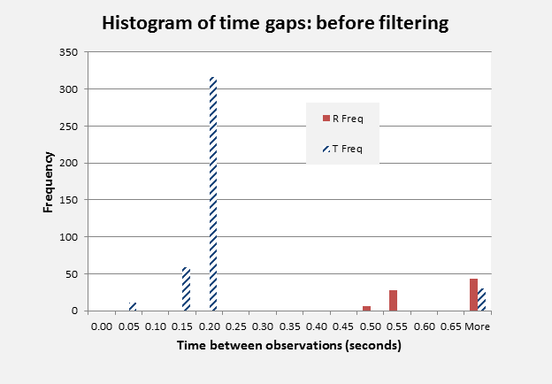
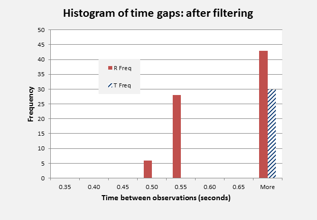
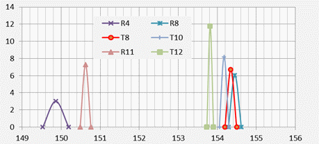
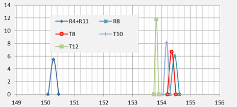
Figure 1: Frequency of time gaps between observations:
before and after filtering. Source: [5](BTO_Tchan) 

Figure 1 gives the frequency of occurrence of time intervals between observations within R- and T-channels, shown separately. It can be noted that the R-channel intervals all exceeded 0.45 seconds and there were no inter-observational time intervals between 0.25 and 0.45 seconds on either channel. Application of the cut-off to exclude BTO data that was within 0.35 seconds of a previous data point (irrespective of channel) only removed K values that were part of a closely correlated sequence of values. These were all on the T-channel and a total of 31 T-channel observations were retained in the time filtered data set, corresponding to the count of 30 time increments shown to the right in Figure 1. The retained T-channel data represented the 20 cluster start points and 11 within-cluster points, and included both of the exceptions noted earlier. No R-channel data points were removed in the process.

Returning to our analysis of the ground data, the time-based filter restored one observation to the calibration data set. Table 3b compares the effects on our estimates of the time interval based T- channel filter with the previous filter based on the SU type.

ATSBX	SU filter	Time filter
Offset δ	4983.3	4980.6
K-bar	-495679.5	-495679.5
Standard deviation of K	29.8	29.6
Count	61	62
Standard error of K-bar	3.81	3.76

Table 3b: Comparison of estimates using alternative filters. Source: [5] (Statistics). All figures in microseconds. 

One additional T-channel data point was brought into the estimation. This had a noticeable effect on the value for the T- channel offset but had no impact on the value for the estimated mean BTO constant. The standard error of the estimate was marginally reduced.

5 Comparison of impacts of PAR5 and ATSBX Satellite Vectors on the mean BTO constant

New satellite vectors became available allowing recalibration to be conducted with the time-filtered reduced data set.  This improved set (PAR5) was obtained from Henrik Rydberg [6] (see also this post). The key statistics are given in Table 4.

	ATSBX	PAR5
Offset δ	4980.6	4980.3
K-bar	-495679.5	-495679.0
Standard deviation of K	29.6	29.6
Count	62	62
Standard error of K-bar	3.76	3.75

Table 4: Comparison of ATSBX and PAR5 using the time interval filtered data set. Source: [5] (Statistics). All figures in microseconds. 

Using PAR5, the optimum T-channel offset for the reduced set of 62 data points was 4980.3 microseconds, a reduction of 0.3 microseconds from the ATSBX value. The new BTO constant was -495679.0 microseconds.  The net result of using PAR5 instead of ATSBX on the BTO constant was a change of 0.4 microseconds, calculated before rounding. There was no appreciable change to the standard error.

6 Comparison of Estimates from Reduced and R-Channel Data Sets

When the optimum value for the T-channel offset is used it is expected that the resulting combined BTO constant would be equal to that obtained from restricting the estimate to the R-channel data alone, but that the standard deviations and standard errors would be different. As the reduced data set only retains eight T-channel data points, the impact of restricting estimation to the R-channel is expected to be modest.

	R-Channel	Reduced
Offset δ	Not applicable	4980.3
K-bar	-495679.0	-495679.0
Standard deviation of K	30.0	29.6
Count	54	62
Standard error of K-bar	4.09	3.75

Table 5: Comparison of R-Channel and time-interval Reduced estimates, based on PAR5 satellite vectors. Source: [5] (Statistics). All figures in microseconds. 

Table 5 confirms that the same estimate for the mean BTO constant is obtained for the Reduced, and R-channel, data sets. The standard deviations are only slightly changed. The standard error of the R- channel data is larger, primarily due to the reduced sample size.

7. A Second Look at the ATSB June Estimate

In section 2 it was concluded that the similarity between the ATSB’s estimated BTO constant given in [4] (Appendix G, Table 2) and our preliminary estimates was fortuitous. Similar values were obtained as our analysis was refined. The topic merits a second look and in this section we seek to quantify how likely the ATSB’s estimate may have been.  We will employ risk analysis to assess the probability of obtaining differences of various magnitudes in the sample mean BTO constant.

The ATSB June estimate of the mean BTO constant was given as -495679(.3) microseconds and was based on only 17 out of 54 R- channel data points. The first decimal place has been calculated from the values in ATSB’s table. However as we have refined our modelling of the satellite location, in order to make a fair comparison we first need to recalculate ATSB’s mean BTO constant with our current set of satellite vectors.

Using the PAR5 satellite vectors, the mean BTO constant for ATSB’s selected 17 data points would be -495680.2 microseconds. This differs from the R-channel mean of -495679.0, reported in Section 6 above, by 1.2 microseconds. It is this 1.2 microsecond difference whose prior probability we seek to assess.

The question to be addressed by the risk analysis is how probable is it that 17 randomly-selected R-channel ground data points would lead to a mean BTO constant that is within 1.2 microseconds of the mean BTO obtained for a population of size 54? A simulation with one million iterations was conducted to obtain the distribution of sample means of BTO constants from random samples of size 17, chosen without replacement from the 54 available data points.

It transpired that a difference of 1.2 microseconds or less would occur for about 15% of the samples. So the odds are clearly against observing a value this close, confirming our initial conclusion that the similarity was fortuitous. On the other hand, 15% is still an appreciable probability, and so this is not an entirely surprising outcome.

Using other outputs from the risk analysis, Table 6 gives the probabilities of observing specific differences in the mean BTO constant, for a range of alternative magnitudes.

Difference in the sample mean K, microseconds	0.5	1	1.5	2	3	4
Probability in a sample of size 17	6.5%	12.9%	19.4%	25.6%	37.6%	48.7%

Table 6: Probabilities of obtaining close mean BTO constant values from random samples of size 17.

Table 6 tells us, for example, that a difference within 0.5 microseconds would occur with a probability of only 6.5%, while a difference that is within 2 microseconds would be expected in about one quarter of the random samples. Reference [7a] contains the original model that was used and requires the Palisade @RISK package. Reference [7b] contains the results of the risk analysis.

Conclusions

In this report we have demonstrated the sensitivity of the magnitude of the T-channel offset to the data set being adopted for calibration, but also that similar values for the BTO constant can be obtained provided T-channel offsets are re-estimated for the dataset being adopted. We have compared our preliminary estimates for the mean BTO constant with those published by the ATSB and obtained a close match with its published findings. However, the smallness of the ATSB’s sample suggests that a wide confidence band should have been placed on its estimate, and the similarity in our estimates of the mean is fortuitous. On the basis on the current analysis, a consistent estimate, with narrower confidence band, would be justified.

We then conducted a review of data from the T-channel, leading to the identification of a reduced data set for subsequent estimation. More robust estimates for the BTO constant were obtained from the reduced data set. We also studied the impact of using a new set of satellite vectors and made a comparison between estimates from the reduced data set and estimates based entirely on BTO data for the R-channel. Using a more extended data set that included the climb and early cruise phase, we also examined how the data reduction process could be refined.

Based on the reduced dataset, using the PAR5 satellite vectors, the mean value for the BTO constant was -495679 microseconds, with a standard error of the order of 4 microseconds. The 95% normal confidence limits for this estimate are from -495671 to -495687 microseconds. Using the improved PAR5 satellite vectors provided an opportunity to revisit the ATSB’s June estimate for the BTO constant. It was concluded that the odds were against ATSB obtaining a value that was within 1.2 microseconds of our current estimate. However the probability is not sufficiently small for this to be a particularly surprising result.

A possible topic for further investigation would be a validation of the mean BTO constant using the aerial data (i.e. data obtained whilst the aircraft was airborne, in the early part of the flight).

Acknowledgement: The authors wish to thank Michael Exner for many detailed comments on previous drafts of this report. Any errors or omissions remain the responsibility of the authors.

References

[1] Exner, M. L. (2014). Derivation of Net L band Propagation Delay and Range from MH370 BTO Values. MH370 Independent Group. Available online at: http://www.aqqa.org/MH370/models/exner/RT_VS_VT_Delay_2014-06-25.pdf

[2] Inmarsat plc UK (2014). MH370 Data Communication Logs. Available online at: http://www.dca.gov.my/mainpage/MH370%20Data%20Communication%20Logs.pdf

[3] Sladen, P. (2014). Consolidated ADS-B logs for MH370.
Available online at: https://github.com/sladen/inmarsat-9m-mro/tree/master/ads-b/

[4] MH370 – Definition of Underwater Search Areas.  26 June 2014. Australian Transport Safety Bureau. Available online at: http://www.atsb.gov.au/mh370/mh370-definition-of-underwater-search-areas.aspx

[5] Hyman, G., and Martin, B. (2014). Microsoft Excel model for BTO constant. MH370 Independent Group. Available online at: http://www.aqqa.org/MH370/models/BTO_constant_GHBSM06.xlsx

[6] Rydberg, H. (2014). PAR5 Vector Set for IOR 3F1, based on vectors in [4]. MH370 Independent Group. Available online at: http://bitmath.org/mh370/satellite-par5-ecef.txt.gz

[7a] Hyman, G., and Martin, B. (2014). Microsoft Excel model with a Palisade @RISK simulation for the mean BTO constant for 17 randomly sampled R-channel BTO constant point-estimates. MH370 Independent Group. Available online at: http://www.aqqa.org/MH370/models/BTO_resample17_ATSB-sim.xlsx

[7b] Hyman, G., and Martin, B. (2014). Microsoft Excel model with a Palisade @RISK simulation for the mean BTO constant for 17 randomly sampled R-channel BTO constant point-estimates: simulation outcomes. MH370 Independent Group. Available online at [41 MB]: http://www.aqqa.org/MH370/models/BTO_resample17_ATSB-simResults.xlsx