The Orbital Debris Collision Hazard for Proposed Satellite Constellations

 The Orbital Debris Collision Hazard for
Proposed Satellite Constellations

Duncan Steel
2015 April 30


Introduction

In my first post here on the calculation of orbital debris collision hazards I wrote the following in connection with reported plans to insert  constellations of satellites into low-Earth orbit (LEO), in the following case at altitude 800 km:

“If these enhancement factors are of the correct order, then the collision probability attains a value of around 5 × 10-3 /m2/year, implying a lifetime of about 200 years against such collisions with orbital debris. This indicates that there is cause for concern: insert 200 satellites into such orbits and you should expect to lose about one per year initially, but then the loss rate would escalate because the debris from the satellites that have been smashed will then pose a much higher collision risk to the remaining satellites occupying the same orbits (in terms of a, e, i). This ‘self-collisional’ aspect of the debris collision hazard I highlighted in the early 1990s.”

The enhancement factors in question are those that elevate the collision probability for any planned satellite above the value I had calculated on the basis of the orbits of the 16,167 objects listed in the Satellite Situation Report in early April. These factors may be summarised as follows: (a) The lack of available orbits for objects that are CLASSIFIED, this potentially increasing the collision probability by 25 to 50 per cent; (b) An increase by a factor of two or three in the collision probability due to the finite sizes of tracked objects compared to the one-square-metre spherical test satellite assumed in my calculations (with the potential impactors being taken to be infinitesimally small); and (c) The overall collision probabilities being higher perhaps by a factor of a hundred due to the large population of orbiting debris produced by fragmentation events that is smaller than the (approximately) 10 cm size limit for tracking from the ground by optical or radar means but nevertheless large enough to cause catastrophic damage to a functioning satellite in a hypervelocity impact.

Herein I consider in more detail two mooted satellite constellations, intended to deliver internet access to the entire globe, and assess the orbital debris collision hazard that they will face; and also the hazard that they would pose to themselves and other orbiting platforms should the plans go ahead.

or


Proposed internet satellite constellations  

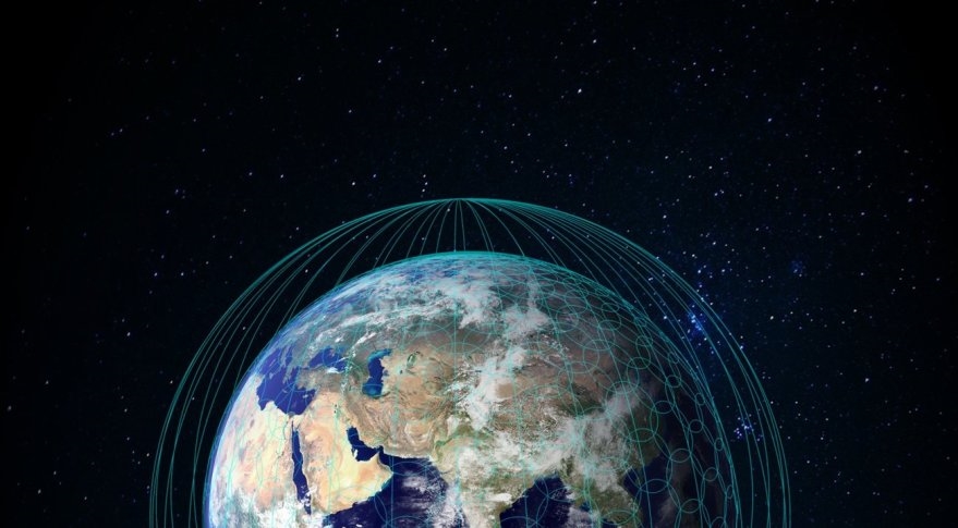
Several distinct satellite constellations have been proposed and are apparently undergoing development, although definitive information is sparse. As an initial illustrative example I will describe WorldVu, a proposal stemming from former employees of Google although subsequently spun off into a new company and rebranded as OneWeb. The original WorldVu plan apparently involved a constellation of 360 satellites in total, 180 each at altitudes of 800 and 950 km, and all having an inclination of 88.2 degrees. At each altitude the 180 satellites would be arranged in nine orbital planes each containing twenty satellites. Shown below is a visualization of just the 180 satellites at altitude 950 km, with the blue access cones beneath each satellite indicating the coverage of Earth’s surface subject to a limitation of the elevation angle from ground to satellite being at least 25 degrees (this being a conceivable limit for ground station access to each satellite).

Strawman_WiFi_Constellation_950km

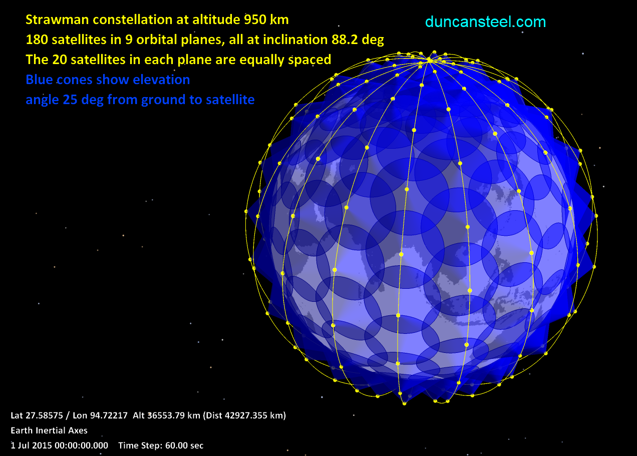
Graphic above: A Strawman satellite constellation of 180 platforms in polar orbits. A movie showing the movement of these satellites in orbit is available for download from here (14.4MB).

My previous posts on the LEO debris collision hazard (here and here) have shown that the collision probability against tracked orbiting objects is particularly high for altitudes 800-1000 km, most specifically for any proposed satellite in a polar orbit (inclinations 80-100 degrees).

Perhaps in recognition of the crowded and congested nature of geocentric space at such altitudes, more recent (i.e. in 2015) proposed satellite constellations have involved slightly higher altitudes, at 1100 km and 1200 km. The two specific constellations that I consider here may be summarised as follows.

  1. OneWeb: 648 (or possibly 700) satellites at altitude 1200 km; individual satellite masses of order 125-200 kg; strategy to evolve to a second-generation constellation of 2,400 satellites.
  2. SpaceX: 4,025 satellites at altitude 1100 km; individual satellite masses 200-300 kg.

Whether or not the above basic information is realistic or not, and whether or not either or both of these proposals go ahead, the two provide pertinent input data for a consideration of the orbital debris hazard that such constellations will face.


Collision probability calculations

I have derived collision probabilities between test satellites and my list of 16,167 tracked orbiting objects as described previously. Although the satellite altitudes (i.e. 1100 and 1200 km) are known, I do not know for certain the proposed inclinations. The previously-promoted WorldVu plan was for an inclination of 88.2 degrees. A graphic from OneWeb shown immediately below indicates polar orbits. Sun-synchronous orbits for altitudes of around 1110-1200 km require an inclination close to 100 degrees. In view of the above I have performed collision probability calculations for those two inclinations, 88.2 and 100 degrees. Note that this means that I have also assumed that the SpaceX constellation would be in polar orbits (and it might well be that lower-inclination orbits would be chosen so as to provide better coverage of low-latitude rather than polar ground locations).

OneWeb_coverage

Above: The proposed OneWeb satellite constellation’s orbits and ground coverage (source: OneWeb website).

In Figure 1 are shown the collision probabilities for test satellites in circular orbits in 50 km steps between altitudes 650 and 2000 km, for the two inclinations discussed above. Purely on the basis of minimising the debris impact risk it is clear that it would be wise to avoid altitudes below 1000 km or even 1050 km.

Sat88and100Pc

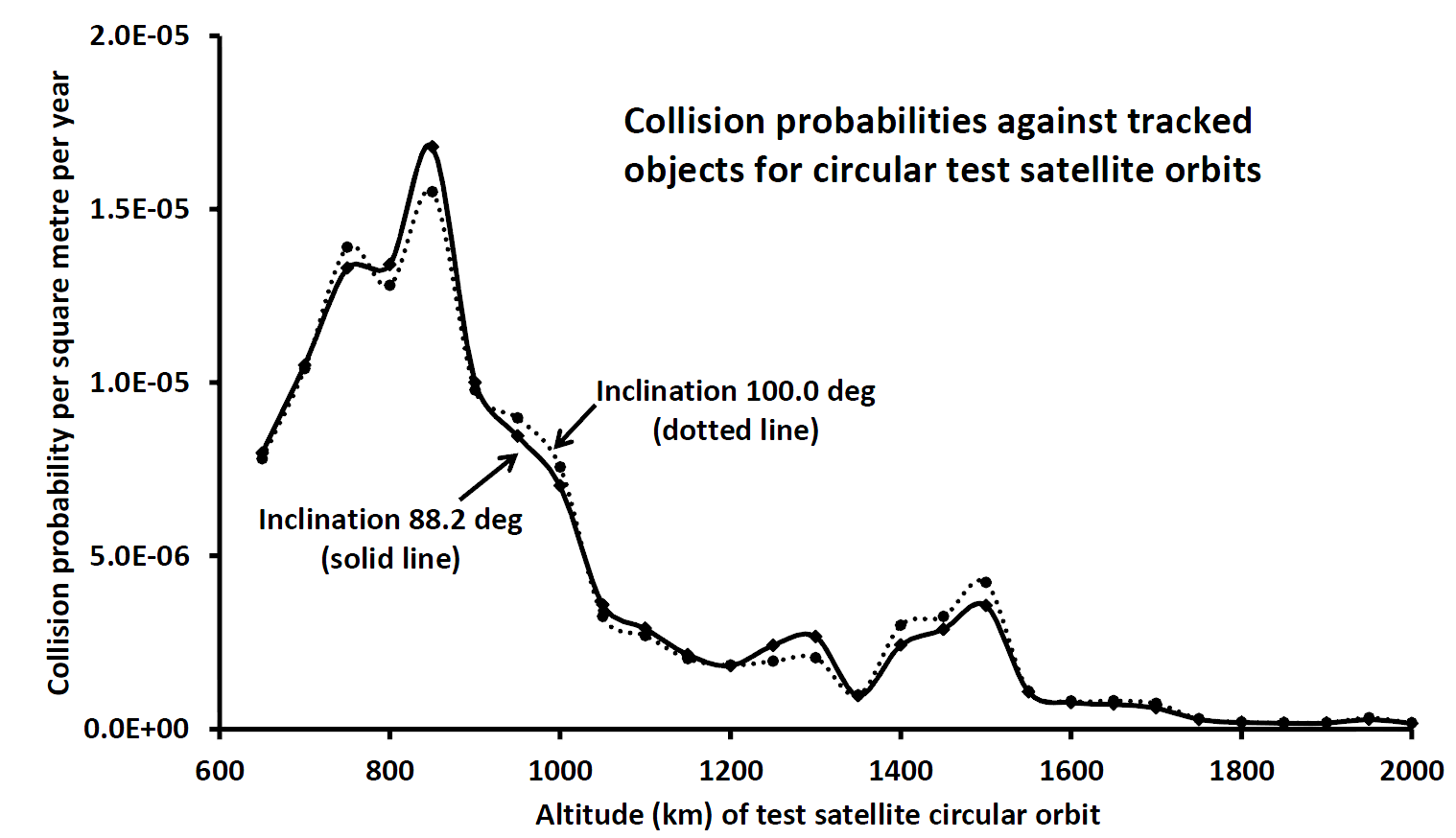
 Figure 1: Collision probabilities against all tracked objects in the publicly-available Satellite Situation Report as a function of altitude for circular test orbits and for two different near-polar inclinations; a spherical test satellite of cross-sectional area one square metre is used, and all possible impactors (the tracked objects) are taken to be infinitesimally small (i.e. the mutual collision cross-section is assumed to be one square metre in every case).

The form of Figure 1 might, in isolation, be thought to imply that there are comparatively few objects whose orbits take them above 1,000 km altitude, and indeed it has been reported in the media that this is one reason for the SpaceX choice of an altitude of 1100 km. However, this is not the case: there are many tracked objects in orbits well above 1000 km. In Figure 2 I plot the numbers of tracked objects with orbits that cross each of the discrete altitudes in Figure 1. Whilst that plot peaks at 850 km with just over 5,000 tracked objects, there are still about 3,000 tracked objects crossing 1100-1200 km, and over 2,000 objects right the way up to altitude 2000 km.

In view of the information in Figure 2 it might seem surprising that the collision probabilities as shown in Figure 1 drop rather quickly at altitudes above 1000 km. The lesson to be learned from this is that mere numbers of objects do not provide a reliable indication of the collision risk: their orbits (and especially their inclinations) greatly affect the formal collision probabilities. It happens that polar orbiters have disproportionately high collision probabilities (with extreme likely impact speeds), and most polar orbiters (e.g. in sun-synchronous orbits) circuit our planet at altitudes below 1000 km.

SatPop

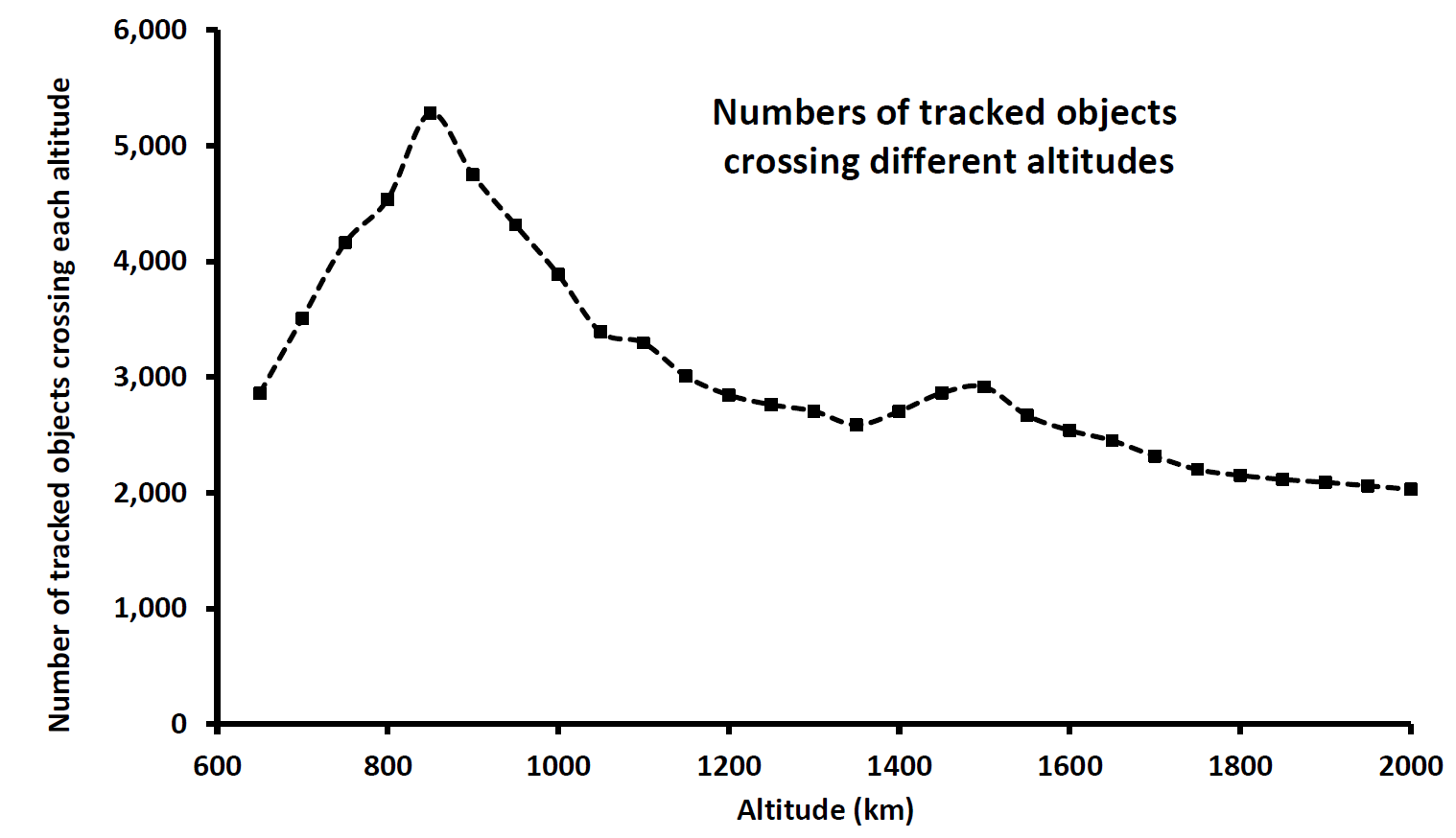
Figure 2: Numbers of tracked objects with orbital paths crossing discrete altitudes between 650 and 2,000 km.

In order to move from a collision probability per square metre per year (as in Figure 1) to a collision probability for specific satellites we need to have some information regarding their size. Although ballpark masses have been stated above for individual satellites in the proposed OneWeb and SpaceX constellations, specific linear dimensions are not known (at least by me!). The graphic below shows an artist’s representation of a OneWeb satellite, and that I have used to estimate that a size of about 5 × 1 × 1 metres is of the correct order.

OneWeb_satellite

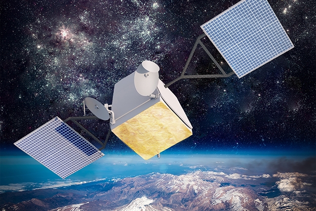
Above: Representation of a OneWeb satellite in orbit
(source:
OneWeb website).

During each orbit the satellites will rotate their solar panels so as to maintain their direction towards the Sun, and this will have the effect of ‘averaging out’ the cross section with regard to debris approach directions. In view of that I will adopt a characteristic cross-section of three square metres for the OneWeb satellites.

Media reports of the masses and planned capabilities of the SpaceX constellation satellites indicate that these may well be larger. For these I will adopt a characteristic cross-section of five square metres.

Regardless of the choice of inclination (88.2 or 100 degrees) the collision probabilities in Figure 1 at altitudes of 1100 and 1200 km are approximately 3 × 10⁻⁶ and 2 × 10-6 respectively, per square metre per year. These lead to the following estimates for the collision probabilities, when the cross-sectional areas of the satellites are included:

OneWeb satellites:         6 × 10-6 per year

SpaceX satellites:             1.5 × 10-5 per year

It is emphasized that these values should be considered to be lower limits on the orbital collision probabilities, due to factors that have been previously mentioned: (i) There is no allowance for CLASSIFIED orbiting objects; (ii) The finite (often large) sizes of other objects will enhance the collision cross-sections by an average of perhaps two or three; (iii) No allowance has been made for small (less than 10 cm) untracked debris items, and these can increase the collision risk by a large amount; note also that the capability to detect and track small debris items falls off with altitude, given that the US DoD sensors are ground-based.

I would have difficulty in making a case for overall enhancements in the collision probabilities due to the preceding considerations being less than by a factor of ten, and quite likely the true enhancement is by 20 to 50. It may only be through statistics of satellite losses that we will be able to obtain a true assessment of the hazard, or else satellite-borne sensors counting the frequency of near-misses by small orbiting debris (plus natural meteoroids).

If one adopts an enhancement by only a factor of ten, perhaps dominated by 1-10 cm untracked debris from disintegrations such as the Chinese ASAT demonstration in 2007 and that of DMSP-F13 just less than three months ago (see my notes in this post), the catastrophic collision probabilities against orbiting debris become:

OneWeb satellites:         6 × 10-5 per year

SpaceX satellites:             1.5 × 10-4 per year

(Note that although the two satellite disintegrations mentioned above occurred at around 850 km, tracked debris fragments from them have attained apogees crossing the altitudes of the above two proposed satellite constellations; and smaller, untracked debris items generally have larger relative speeds, making them more likely to attain higher apogees. I also note that at this stage the cause of the observed disintegration of DMSP-F13 is unknown, and it might well have been due to an impact by a fragment of the Chinese ASAT target, Fengyun-1C.)

Next I multiply the above probabilities by the number of satellites in each proposed constellation (648 and 4,025 respectively), to obtain an estimate of the loss rates:

OneWeb constellation: 0.04 per year
(one catastrophic collision per 25 years)

SpaceX constellation: 0.6 per year
(one catastrophic collision per 20 months)

A note here on collision speeds: the most likely impact speeds for mutual collisions between polar orbiters at these altitudes (1100-1200 km) are above 14 km/sec.


Implications

The above estimated satellite loss rates due to debris collisions might be considered to be tolerable, but there are other implications. The most important matter, which stems directly from the sorts of calculations performed here, is that any satellite (or other associated object such as a rocket body) in a constellation that suffers a catastrophic fragmentation event immediately elevates the collision hazard for all other satellites that remain in similar orbits. Essentially, the collision probability between two orbiting objects goes up markedly when they have similar orbits, in terms of their perigee/apogee altitudes and inclinations (or a, e, i).

As an example, consider one satellite in the proposed SpaceX constellation which undergoes a disintegration due to being hit by some random piece of orbiting debris. The figures above indicate that such an event is to be expected within the first two years of the deployment of the proposed constellation (and by the time that the constellation is deployed the orbital debris hazard will certainly be worse, not better). Let us assume that the satellite dry mass is 250 kg. Observations of the mass distributions of objects fragmenting in orbit, and indeed deliberate (chemical) explosions of spare satellites in laboratories, indicate that more than 10,000 fragments with masses above 1 gram are to be expected, and each will be moving on an orbit distinct from the parent satellite but nevertheless on quite a similar path. Each of those fragments now poses an impact hazard to all other satellites in the constellation: they are no longer subject to station-keeping, and they are no longer moving in step with the functioning satellites.

(There is an entirely different way of looking at this, that astrophysicists will likely understand. To first order one may say that if there are n satellites in a constellation then the collision hazard they pose to themselves goes up as  rather than n.)

Assuming an original satellite orbit to be circular at 1100 km, and the debris initially to have perigee and apogee heights spread a few kilometres above and below that, the collision probability for each fragment with each of the other satellites is found to be about 5 × 10-7 per year. For 10,000 fragments capable of colliding with 4,000 functioning satellites the collision rate is then:

5 × 10-7  × 10,000 × 4,000 = 20 per year

What happens, of course, is not that twenty satellites per year are lost, but rather a rapid cascade occurs with a proliferation of debris in similar orbits obliterating all functioning satellites and leaving that region of LEO unusable for a very long time. This is the Kessler syndrome writ large.


Final comments

Although in this series of posts on orbital debris I have been making use broadly of test satellites assumed to be spherical, that is a non-necessary simplifying assumption. In fact it is possible to derive face-dependent impact probabilities and indeed impactor speed distributions for satellites that maintain their orientations during an orbit, and I not only have software to do this, but have exercised it in the past. Most of my results from the use of that software has not been published, either here or elsewhere; I am intending to prepare other posts for publication here, illustrating the sorts of understandings that can be derived (and it is only through understanding a problem that we can equip ourselves with the wisdom to act and react in certain ways).

rr

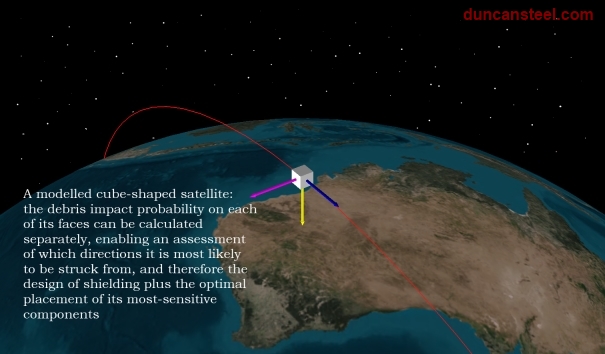
There are at least two good reasons to make use of such software when planning future satellites. The first is so that a proper assessment of the orbital debris hazard can be made, making use of the real size and shape of the satellite (including its solar panels) rather than an assumed spherical form, as here. The second reason is that, at least for very small debris items (and indeed meteoroids and interplanetary dust), knowledge of the most likely arrival directions and speeds would enable appropriate shielding to be installed, and also the arrangement of the more sensitive parts of the satellite to be planned so as to minimise the overall mission risk. One cannot entirely obviate the orbital debris collision risk, but one can make judicious decisions on how to minimise it once one is well-informed.


The Orbital Debris Collision Hazard for Satellites in Geostationary Orbit

The Orbital Debris Collision Hazard for
Satellites in Geostationary Orbit

Duncan Steel
2015 April 29

Introduction

In my two previous posts (here, and here) regarding the orbital debris collision hazard I have been considering only test satellites in low-Earth orbit (LEO). In this post I turn my attention to satellites in geostationary orbit (GEO); that is, satellites in orbits that have periods of one sidereal day (i.e. altitudes near 35,800 km) and are in near-circular (i.e. low eccentricity) paths close to the equatorial plane (i.e. low inclination). Such orbits are used for many communications satellites, and are sometimes termed Clarke orbits.


A crude estimation of the typical collision probability in GEO

In principle it is straightforward to derive an estimate of the collision probability with space debris for a satellite in GEO. Consider the diagram below. The white circle shows the orbit of a geostationary communications satellite: there are many such satellites in GEO, but they remain in set positions due to their operators performing station-keeping burns/manoeuvres and so cannot collide with each other. Even a GEO satellite which is no longer under control only has a small drift speed (much smaller than the GEO orbital speed of  3.075 km/sec) and so the risk of inter-satellite collisions is very small, if we are considering only true geostationary satellites.

GEO hazard

This is not true, however, for orbiting objects that cross the GEO altitude. The red ellipse in the diagram is intended to represent a rocket body in a geostationary/geosynchronous transfer orbit, having performed its purpose in carrying a GEO satellite to the necessary altitude. That defunct rocket body will pose a collision hazard to all functioning satellites in the geostationary band, as its argument of perigee and longitude of the node precess under gravitational perturbations due to the Moon and the Sun, and also the Earth’s oblateness (dependent upon the altitude of its perigee).

Imagine a sphere with radius (r) equal to the distance of the geostationary band from the centre of the Earth (about 42,000 km). That sphere has an area of 4πr2. The rocket body, having an apogee above the geostationary band as shown, crosses that band twice per orbit, giving it two chances to hit that one particular communications satellite. If we estimate the mutual collision cross-section to be 100 square metres, then the probability of a collision is given by 2 × 100 / 4πr2 which is a shade less than one part in 1014 per orbit of the GTO object (the rocket body). That GTO will have a period lower than one sidereal day, perhaps about 15 hours, or one part in 584 of a year, so that our estimate of the mutual collision probability becomes about 5 or 6 × 10-12 per year.

To put that figure into some perspective, the universe is about 13.8 billion years old, and so a mutual collision would have a probability of occurrence of less than ten per cent over such a timescale. (Of course, the solar system is only about one-third the age of the universe; and over such phenomenal timescales all manner of other things happen.)

This, however, was a calculation for a mutual collision between only one pair of orbiting objects. The reality is that there are hundreds of satellites in geostationary orbit; and hundreds of rocket bodies and fuel tanks and other debris items crossing the GEO altitude, so that a more sophisticated assessment of the collision hazard is warranted.


Specific example orbits

The Inmarsat 5F2 communications satellite was launched on 2015 February 01 and inserted into geostationary orbit. The Briz-M rocket booster that was used to carry it to its final altitude remains in a GTO similar to that shown in the preceding diagram. Orbital parameters for the two objects in question are shown in the table below; note that the inclination and eccentricity of Inmarsat-5F2 in particular will vary from day-to-day and week-to-week under the influence of gravitational (and radiation-induced) perturbations, plus station-keeping burns by the operating company.

Name International Designator Satellite Catalogue Number (SCN) Perigee altitude (km) Apogee altitude (km) Eccentricity Inclination to the Equator (degrees)
Inmarsat-5F2 2015-005A 40384 35,551 36,029 0.000165 0.0338
Inmarsat-5F2 Rocket Body 2015-005B 40385 2,775 63,223 0.767648 27.6213
Inmarsat-5F2 Fuel Tank 2015-005C 40386 355 14,849 0.518453 50.7385

The final line in the table, for the fuel tank left in a lower orbit, plays no further part in the present calculations and is included simply for completeness. The orbits of the first two objects are shown in the graphic below, with three views being given so as to indicate the three-dimensional nature of the geometry. In addition a short movie portraying the movements of the two objects over five days is available for viewing and download from here (1.44MB).

I3F2

Graphic above: The orbits of the Inmarsat-5F2 satellite (in a near-circular geostationary orbit) and also the rocket body that carried it there, that rocket body (labelled I5F2RB above) having been left in an orbit with eccentricity near 0.77 and a perigee altitude of a few thousand kilometres. 

Using the orbital parameters listed above I can now calculate the separate collision probabilities involving (a) Inmarsat-5F2 itself; and (b) the Briz-M rocket body used to carry Inmarsat-5F2 to its geostationary orbit, against all objects in the tracked orbiting object catalogue. In a previous post I described the list of 16,167 tracked items that I have been using in calculating collision probabilities. Again using that list I have derived the following results:

Object Number of tracked objects crossed by the I5F2 objects  Net collision probability per square metre per year
Inmarsat-5F2 1,543 3.06 × 10-8
Inmarsat-5F2 R/B 3,763 1.15 × 10-9


Discussion

The collision probabilities derived above are in units of per square metre per year, and are based on a model test satellite in each case having a spherical shape and a geometrical cross-section (and therefore collision cross-section) of one square metre. Of course, the actual objects in question do not have such a size and shape.

The two are shown in the graphic below (the source of which is here). The Briz-M booster might be modelled as being near-enough to spherical for present purposes, with a characteristic size (diameter) of almost five metres, and so a cross-sectional area of about 20 square metres.

I5F2_and_Breeze-M

Graphic showing the Inmarsat-5F2 communications satellite (upper right) and the Briz-M rocket booster (centre). Courtesy Khrunichev.

The Inmarsat-5F2 satellite is much larger. Once its solar cells were deployed it attained a greatest linear dimension of 33.8 metres, and the thermal radiators and antennas that fold out from the main bus render linear dimensions of 8.08 metres. Looking at the satellite from orthogonal views its greatest cross-sectional area is therefore about 270 square metres, and its smallest about 65 square metres.

During its orbit around the Earth the satellite rotates its solar cells so as to keep these pointing towards the Sun, and the effect of this is to ‘average out’ the cross-section from the perspective of potential colliders such that again we might approximate its collision cross-section in terms of a sphere with a cross-sectional area of about 150 square metres, as a rough estimate.

Using that as a collision cross-section one derives a collision probability for the Inmarsat-5F2 satellite of about 5 × 10-6 per year (i.e. 150 × 3.06 × 10-8) and so a characteristic event rate of one collision per 200,000 years.

This value, however, is misleading: as noted earlier, most objects in the geostationary belt are moving in step, making it infeasible for them to collide with each other. One approach I could take here would be to sort through the 1,543 objects crossing the orbit of Inmarsat-5F2 and weed out those that are also truly geostationary or geosynchronous, making collisions with each other impossible in the present epoch, but it is sufficient to say simply that the true collision probability against other tracked objects is likely an order of magnitude less than the value calculated here (and so around 5 × 10-7 per year, or a timescale of two million years).

Turning to the Briz-M rocket body, there is nothing to protect it from collisions with objects in the geostationary belt (or anywhere else). The collision probability for this object is therefore about 2.3 × 10-8 per year (i.e. 20 × 1.15 × 10-9) and the characteristic collision time is of order 40 million years.

In my first post here on orbital debris I discussed three different ways in which the ‘true’ collision probability could and would be higher than my calculations indicate, these ways being:
(i) The Satellite Situation Report and Two-Line Elements that are publicly-available do not include any CLASSIFIED orbits, these comprising almost 800 objects compared to the 16,167 in my listing used in these calculations;
(ii) Many of the tracked objects are larger than my model spherical satellite of cross-sectional area one square metre, so that the true collision cross-section for specific cases will be substantially larger than one square metre; and
(iii) The tracked objects are larger than about 10 cm in size, else they are not detectable with the ground-based optical and radar sensors employed by the U.S. military to keep tabs on anthropogenic orbiting objects, but fragmentation events such as remnant fuel explosions and hypervelocity collisions will produce many orbiting objects smaller than that 10 cm limit.

Taking each of these considerations in turn:
(i) There are certainly various CLASSIFIED payloads in geostationary orbit, and rocket bodies used to take them there also have GEO-crossing paths, but the effect of including these is unlikely to boost the derived net collision probability for objects in geostationary orbit by more than 50 per cent;
(ii) The communications satellites in GEO tend to be the largest objects in such orbits (unlike in LEO, where the International Space Station, the Hubble Space Telescope and various classified surveillance platforms dwarf most other satellites) so that the appropriate collision cross-sections to use are indeed the sizes of the communications satellites themselves, with areas dominated by solar cell arrays and typically being 100-300 square metres; and
(iii) There is very little small debris in orbits crossing the geostationary band, and so the enhancement in the collision probability due to sub-decimetre projectiles is small.

Overall my analysis leads to an expectation that the individual lifetimes of satellites in the geostationary band against catastrophic collisions with artificial space debris are of order millions to tens of millions of years.


Conclusions

I will now repeat what I have just written: the individual lifetimes of satellites in the geostationary band against catastrophic collisions with artificial space debris are of order millions to tens of millions of years.

If this conclusion is correct then, from the perspective of satellite protection and safety, there is no real need to boost defunct satellites into higher orbits, as is current practice. Indeed one might argue that to do so may have the effect of increasing the collision hazard: in any orbital manoeuvre there is a finite likelihood of something going wrong, perhaps with disastrous consequences. For example, re-igniting a rocket booster attached to a communications satellite, when that booster had been dormant for a decade or more since the satellite was placed in its desired station, might  lead to an explosion and thus the spreading of myriad pieces of debris around the geostationary belt with high relative velocities. It would be better to leave the satellite as it was, simply closing it down until future generations with better technical capabilities can clear it up.

If the debris impact timescale for geostationary orbits is indeed of order millions of years, the collisional impact risk for satellites in that high-altitude band is dominated by the flux of natural meteoroids. I will say nothing more on that subject here, and simply refer the reader to a recent report on the subject.


The Last 15 Minutes of Flight of MH370

The Last 15 Minutes of Flight of MH370

Brian Anderson
Report prepared 2015 April 24


 Introduction

Determining what happened to MH370 during the last 15 minutes of flight is difficult, given the limited information available, yet it is important to arrive at some estimates of the aircraft altitude and path during this time. The path is needed in order to establish where the end point might be.

At the time of the Independent Group’s (IG) September 26 statement last year, the information available to help with the analysis of this period was limited to the satellite-derived BTO and BFO data at 00:11 and 00:19 UTC (on 2014 March 08), and the expectation that the engine failures with fuel exhaustion would not occur at precisely the same instant in time.

It was expected at that stage that knowledge of the engine Performance Degradation Allowance (PDA) figures would provide evidence as to which engine failed first, and also enable the remaining flight time before the second engine failed to be determined. Unfortunately the PDA information has not been made public by Malaysia Airlines.

The analysis of several simulation runs in a certified B777 level 4 simulator showed that knowing which engine fails first, and hence being able to determine the direction of the Thrust Asymmetry Compensation (TAC) deflection at the time of the second engine failure, is not a predictor of the flight characteristics of the aircraft following the second engine failure. Hence, knowing the PDAs is not immediately helpful in this regard (i.e. knowing which engine first ran out of fuel is not a necessity here). Rather, the flight characteristics, and in particular the propensity of the aircraft to bank into a turn immediately following the second engine failure, is a function of precisely how the aircraft was trimmed immediately before the first engine failure. The simulator trials showed that seconds after the second engine failure the TAC is reset to the cruise rudder trim position.

We know that each B777 aircraft is subtly different (as are most other aircraft) with respect to rudder trim in particular. One might say that they may be slightly ‘bent’ in terms of aerodynamics.  Some require a little left trim, some a little right, and some require neither in order to fly straight. In addition, individual pilots often adopt slightly different regimes in order to manage the trim (TAC) requirements. Without knowing how this particular aircraft handled historically – and even if we did know – it may not be possible to say with certainty if the aircraft would depart into a turn to the left or to the right following the second engine failure.

In performing the analysis presented in this paper I have made the following necessary assumptions:

  • There was no manual intervention to control the aircraft during the last 15 minutes of flight;
  • The aircraft was flying on autopilot during its passage south over the Indian Ocean until the second engine failure;
  • The flight path is similar to the path discussed in the IG statement dated September 26 (and also a number of other independently-derived flight paths ending at similar latitudes, so that the precise flight path taken over the Indian Ocean is not significant here);
  • The B777 level flight simulator runs previously studied by the IG (per Mike Exner) deliver a valid representation of how MH370 would be expected to have behaved near the end of its flight.


Fuel Data

With the release of the Factual Information statement by the Malaysian Safety Investigation Team on 08 March 2015 [reference 1], new information became available which enabled more analysis of the fuel consumption rates and better estimates of the engine failure timings, without requiring specific knowledge of the PDAs. This at least enables us to say with some certainty that it was the Right engine that failed (ran out of fuel) first.

When the first engine fails the TAC is immediately set to trim the aircraft to fly straight, and the auto-throttle increases thrust in order to maintain air speed and altitude, as far as possible.

The ATSB, in its 26 June 2014 report [2], described the Satellite Data Unit (SDU) power up process and concluded that the 0019:29 log-on would have occurred three minutes and 40 seconds (+/- 10 seconds) following the second engine failure, and that the autopilot would have been disengaged for this period due to the interruption in electrical power. The SDU boot-up and final log-on is assumed to be a result of an automatic Auxiliary Power Unit (APU) start due to the loss of both electrical generators driven by the jet engines. The time required for the entire process, from loss of the second engine until the log-on, is 3m40s. This time was confirmed during the B777 flight simulator trials mentioned previously.

Note that the APU is supplied from the left main (fuel) manifold, and will continue to run only for as long as there is sufficient fuel in the fuel lines to the APU (given that the fuel tanks are empty, resulting in the jet engine failure). It is not surprising therefore that the final communication received from the aircraft was at 00:19:38, a possible cause being complete loss of power again, as the APU shut down. (An alternative explanation for the incomplete log-on might be mis-direction of the satellite communications antennae due to a spiral dive;  however the receiver power indications provided by Inmarsat [3] remain stable throughout all signal exchanges, and so this possibility seems less likely.)

The possibility that the aircraft impacted the sea at or very shortly after this time (00:19:38) should not be ignored: an implication of this would be that at that time the aircraft was at a low altitude, affecting the calculated position of the 7th/final ping arc, and therefore the search region for wreckage on the sea floor. Taking the aircraft altitude to be near zero at this time rather than at 35,000 feet has the effect of shifting the 7th ping arc by about 10 km to the northwest; this is discussed in more detail below.

A separate analysis of the fuel data is being undertaken within the IG [4] and it is sufficient to recognize here that the rate of fuel consumption rate for both engines combined for the remainder of the flight, from 17:07 through to 0019:29, is an average of about 6,072 kg/hr, (13,386 lbs/hr), and hence significantly lower than that shown for the take-off and climb phases of the flight as reported in the Factual Information [1], Appendix 1.6B. It is expected that the difference in fuel consumption rates between the two engines will be lower too (information in the Factual Information report indicates differences of 1.9 and 1.3 per cent, for take-off and climb: reference 4), and for the purpose of the ongoing discussion I have assumed, based on a simplified analysis, that this difference is 0.8 per cent. Using this figure it is possible to deduce that the Right engine failed close to, and perhaps a few seconds before, 00:11 UTC on 2014 March 08.


Flight path after the first engine failure

The simulator trials mentioned earlier illustrated clearly that following the first engine failure the auto-throttle increased thrust in the remaining engine, altitude was maintained, and the (longitudinal) pitch increased as the speed reduced so as to provide adequate lift. The deceleration observed was noted, and the Indicated Air Speeds (IAS) were converted to True Air Speeds in Knots (KTAS) for illustration in Figure 1, below. The observed trend is linear, with a deceleration of approximately 19 knots per minute. (dy/dx = -0.315 ´ 60 = -18.9). A deduction from this result is that the aircraft would still have been well above the best single engine speed and would have continued to fly at the same altitude for some minutes after the engine failure.

Anderson Fig1

Figure 1: Deceleration after first engine failure

The flight dynamics are such that although drag and the available thrust are lower at higher altitude, the minimum drag speed also increases. Hence, coincident with one engine failing, we would expect deceleration to commence immediately and a reduction in altitude to begin as the minimum drag speed is approached. This was not observed in the simulator trials commencing at FL350 (Flight Level 350, nominally 35,000 feet but in actuality the geometric altitude depends on the atmospheric temperature and pressure). In fact the speed continued to decrease (below the minimum drag speed) without a descent being automatically commenced, but the ensuing part of the simulator trial was perforce cut short by the failure of the second engine. The speed (and time) at which MH370 would have begun to descend is therefore unknown from the simulator trial.

Turning back to what we know about the actual flight, the BFO at 00:11 suggests that at that instant the aircraft was descending at about 250 feet per minute. Together then, the BFO descent rate, the estimated time of the Right engine failure, and the simulator trials, may all be reconciled if the altitude was greater than FL350, in which case it is possible that a shallow descent commenced just prior to 00:11.

The appendices in the ATSB report [2] provide an indication of possible vertical descent rates resulting from loss-of-control events at high altitude. Descent rates of greater than 20,000 feet/min have been observed.

At the rate of speed (and altitude) reduction observed in the simulator trials, and because the aircraft is observed to be within a normally-expected flight envelope, it seems clear that the aircraft would still be close to FL350 (or higher) at the time the second/Left engine failed, at 00:15:49 (+/- 10 seconds). If, as a result of total loss of control at that time (autopilot failure due to interruption of electrical power) it happened that the aircraft impacted the sea at 00:19:38, the average descent rate would have been about 9,500 feet/min, which is well within the observations referenced in the preceding paragraph.

An immediate conclusion should be drawn at this point. Taking a conservative view (conservative, that is, in terms of the plausible distance travelled from the 6th ping arc at 00:11), the 7th arc position calculation should assume that the aircraft was at or near sea level (the surface of the reference ellipsoid) at time 00:19:38, and hence only a little above sea level at 00:19:29, and descending rapidly. At the latitudes of interest this will position the 7th arc at a distance of about 56 nm from the 00;11 arc along the 186 deg (from True North) azimuth in the vicinity of a latitude of 38 degrees South.

Assuming that the deceleration is a linear function, as observed in the simulator trials, the distance travelled from time 00:11 until the Left engine flames out can be calculated. For a range of speeds at 00:11, and assuming that at that time the aircraft was exactly on the 00:11/6th ping arc, the distances are illustrated in Figure 2, below.

Anderson Fig2

Figure 2: Distance travelled from 00:11 before second engine failure

Assuming a ground speed of 480 knots at 00:11 (equivalent to a wind-corrected KTAS of about 500 knots), and noting that this is likely to be an optimistic value since various IG path models suggest ground speeds between 429 and 455 knots at this point, and with a linear deceleration of 19 knots/minute, the ground speed at 00:15:49 would have been 389 knots, and the distance travelled from the 6th arc at 00:11 is 35nm (nautical miles). On an azimuth of 186 degT this will put the aircraft 21nm short of the 7th arc calculated at sea level for when the Left engine fails. Continuing with that rate of deceleration in a straight line (allowing for the effect of wind following the second engine failure), the total distance covered before 00:19:29 is 56 nm, which is just on the 7th arc calculated at sea level, but 6nm/10km short of the 7th arc at FL350.

 Continuing deceleration after the Left engine fails is not a certainty. It is possible that the speed may increase, since it is governed primarily by the relationship between the drag and the component of the aircraft weight acting down the flight path. With the assumption that there is no further deceleration after the Left engine fails, then in 3m 40s the distance covered is 24 nm and hence the aircraft is capable of reaching the 7th arc calculated at sea level, but still not capable of reaching the (FL350) 7th arc at 00:19:29, on the 186 degT azimuth.

As a comparison it is useful to test the outcome assuming a lower ground speed, say 429 knots (rather than 480 knots) at 00:11, and assuming the same rate of deceleration. In this case the ground speed at 00:15:49 would be down to 338 knots, and the distance travelled from the 6th arc at 00:11 would be only 31nm, which is 25nm short of the 7th arc calculated at sea level. In order to reach the 7th arc in a straight line on the same 186degT azimuth, a linear acceleration of approximately 50 knots per minute would be required, reaching a ground speed of 485 knots at 00:19:29. This seems unlikely, and indicates a likelihood that the speed at 00:11 was greater than 429 knots. Perhaps even more likely is the possibility that the aircraft turned towards the 7th arc at the time of the second engine failure.


Flight path after the second engine failure

Observations from the simulator trials suggests that following the failure of both engines the aircraft will bank into a turn almost immediately. The direction of the turn, and perhaps the rate of the initial turn, is a function of precisely how the aircraft was trimmed immediately before the first engine failure, and this is of course unknown. However, the observation that the aircraft may not be capable of reaching the 7th arc if that is assumed to be at 35,000 feet (as discussed above) may help in reaching a conclusion here.

For example, if the aircraft banked and turned to the right after the Left/second engine failed, then with the speed profile examined above, commencing at 480 knots at 00:11, it would not be possible to intercept the 7th arc until after 00:19:29, and even then the turn radius would have to be greater than about 48nm to intercept the arc at all.

Alternatively, if the aircraft banked and turned to the left after the Left/second engine failed then an intercept with the 7th arc at 00:19:29 is possible, but only if the turn radius is between 8 and 10 nm. At the assumed speed at which the turn commenced the required bank angle is approximately 15 degrees. Figure 3, below, illustrates these possibilities.

Anderson Fig3

Figure 3: Illustrating possible tracks after second/Left engine failure

The simulator trials illustrate that after entering a banked turn, even one with a bank angle as shallow as 15 degrees, the aircraft does not recover to a wings-level attitude. Rather, over a period of about three minutes, and interspersed with possible phugoids, the bank angle will continue to increase until the aircraft enters a spiral dive. At that point the bank angle may have increased to 90 degrees, the aircraft may have rotated through three complete turns, the aircraft speed with respect to the air would exceed the normally-allowed maximum operating speed (VMO), but not necessarily have increased beyond maximum Mach operating speed (MMO) at that altitude so that it would likely not have suffered severe structural damage, and the descent rate would be up to 15,000 feet/minute. A high-speed uncontrolled impact with the sea would be inevitable.

Note that a descent rate of 15,000 feet/minute at the airspeeds of interest requires an aircraft track dipping only about 20 degrees below the horizon. More extreme descent rates are certainly possible.


Conclusions

Based on this analysis one may conclude that:

  1. It is only with ground speeds greater than about 440 knots at 00:11 that it is possible subsequently to reach the 7th arc at sea level at all;
  2. Following the Left/second engine failure, the aircraft very likely entered a turn to the left, a turn which developed into a spiral dive over the course of a few minutes resulting in a high speed impact inside the 7th arc as calculated for sea level.

It is clear from this analysis that establishing precisely where the 7th arc is located is very important from the point of view determining the path of the final few minutes of flight, and the underwater search strategy to be used. Based on the corrected BTO (18,400 microseconds) at 00:19:29 provided by the ATSB (2), the advisable position would be to establish the 7th arc at the surface of the reference ellipsoid (i.e., sea level) and not at high altitude (say 35,000 feet) the distinction between these shifting the 7th arc by about 6nm/10km.


Acknowledgements

 I thank members of the Independent Group (IG) for the active discussion, and contributions, which have greatly helped me to present this analysis and to arrive at the above conclusions. It is hoped that these will assist the official search teams in their identification of where to concentrate their efforts to achieve the highest likelihood of timely success.


References

[1]       Factual Information: Safety Investigation for MH370, published 08 March 2015, Malaysian ICAO Annex 13 Safety Investigation Team for MH370, Ministry of Transport, Malaysia.

[2]       MH370 – Definition of Underwater Search Areas, 26 June 2014 (updated 18 August), ATSB Transport Safety Report.

[3]       The Search for MH370, Journal of Navigation, September 2014, authors Chris Ashton, Alan Shuster Bruce, Gary Colledge and Mark Dickinson (Inmarsat).

[4]       Fuel Burn Analysis, spreadsheet by Mike Exner, April 2015. (Note that this link to Exner’s spreadsheet was added on 2015 June 20.)