Autopilot Flight Path BFO Error Analysis

Yap Fook Fah

2015 March 24

(Updated 2015 April 20 to make the BTO and BFO Calculator available online: see reference [4] added at the very end.) 

A downloadable PDF of this report (867 kB) is available here.

1. Background

This report presents a Burst Frequency Offset (BFO) data error analysis of the end-game flight path of MH370 constrained by certain autopilot flight modes. The analysis is broadly similar in approach to that outlined in the ATSB reports [1, 2], but from which crucial quantitative results are not available for independent study.

Recall that the current search area is mainly defined by a compromise between two methods of analysis: “Constrained Autopilot Dynamics” (CAD), and “Data Error Optimisation” (DEO), as outlined in [1].

The CAD method assumes that the flight, at least after 18:40 UTC, was on some autopilot mode, and its range is limited by the amount of remaining fuel and aircraft performance. The ATSB report did not specify the time and location of the final major turn to the south. Further, the report did not provide details on how the generated paths were scored according to their “statistical consistency with the measured BFO and BTO values” [2].

In contrast, the DEO method does not take into account the flight mode, but simply seeks to rank a set of curved flight paths according to the deviation of the calculated BFO for each candidate flight path from the recorded values at the arc crossings after 18:40 UTC.

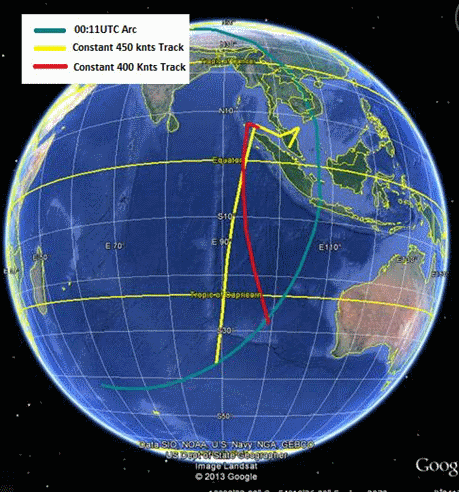
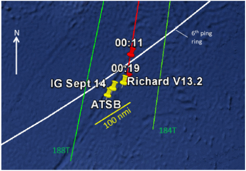
One problem is that the results from the two analyses are not quite consistent with each other. In particular, the DEO results imply that paths ending in the southern half of the CAD probability curve should be ranked much lower and be given less weight. In consequence, this has led to a compromise in the definition of the search area: “Area of interest on 0019 arc covers 80% of probable paths from the two analyses at 0011 …” [1]. This has the effect of shifting the search region further north than if only the CAD results were considered (see Figure 1 below).

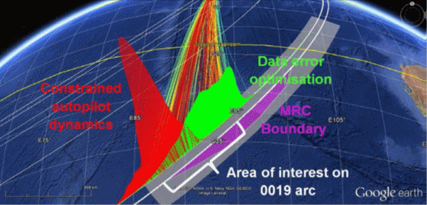
Figure 1: Defining the search area (from reference [1]).

 

2. Objective

The objective of the present report is to reconstruct the end-game flight path BFO data error analysis with autopilot constraints, so as to obtain quantitative results for further evaluation and comparison with other types of analysis.

 

3. Methodology 

• A set of flight paths is generated starting from different locations on the 19:41 arc, each location being reachable from the last known radar position at 18:22 with the aircraft flying at feasible speeds.

• Each path is a rhumb line (or loxodrome) corresponding to a constant true track autopilot mode. The exercise is repeated assuming great circle paths (geodesics). The WGS84 model for the shape of the Earth is used.

• Each path is assumed to be flown at constant altitude. The exercise is repeated with an assumed rate of descent starting at 00:11 UTC (2014 March 08) that minimizes the BFO error.

• All paths cross the arcs at the recorded times, and therefore match the Burst Timing Offset (BTO) values exactly.

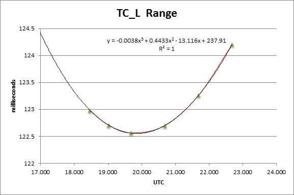
• The ground speed is allowed to vary. The speed profile is derived using a cubic polynomial function fitted over the five points at 19:41, 20:41, 21;41, 22:41 and 00:11. Integration of the speed over time gives the correct distance values at the arc crossings.

• A BFO fixed frequency bias of 150.26 Hz is used [3].

• The BFO values at the five arc crossings are calculated and compared to the recorded BFO values. The root-mean-square (RMS) error for each path is then calculated.

 

4. Results

Figures 2 through 5 are based on the paths southwards after 19:41 being rhumb lines (i.e. loxodromes), whereas Figures 6 and 7 are based on the modelled paths being great circles (i.e. geodesics).

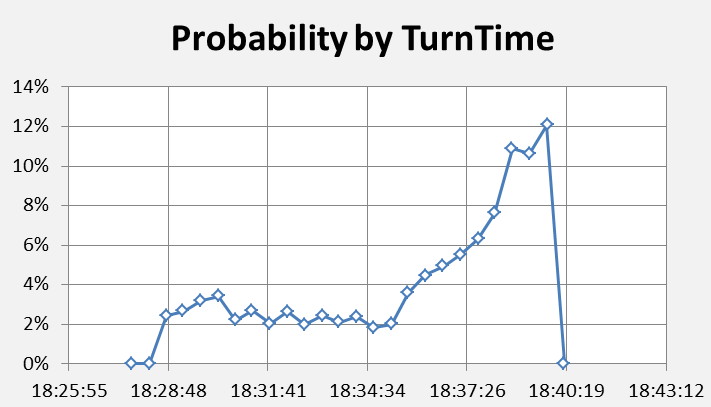
Figure 2 shows, as a function of the assumed aircraft latitude at 19:41, (a) the variation of the minimum RMS BFO error; and (b) the latitude attained at 00:19, based on the rate of descent at 00:19 being optimized (i.e. the BFO value at that time being fitted).

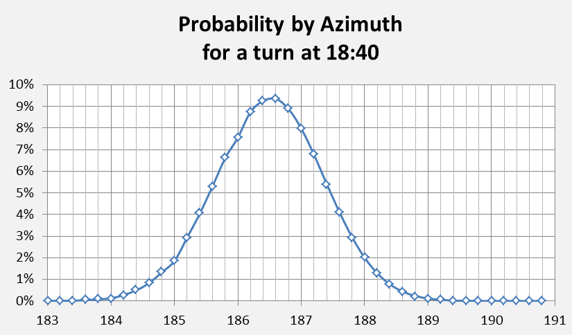
Figure 3 is similar to Figure 2, but represents the azimuth of the derived rhumb line path from the position at 19:41.

Figures 4 and 5 are similar to Figures 2 and 3 except that they result from assuming no descent (a level flight) at 00:11.

Figure 6, for a great circle path as described above, is similar to Figure 2 in that the minimum RMS BFO error and the latitude attained at 00:19 is depicted, based on the rate of descent at 00:19 being optimized.

Figure 7 is similar to Figure 3: the minimum RMS BFO error and the latitude attained at 00:19 is depicted, based on no descent (a level flight) at 00:11.

Obviously there are no graphs/figures for constant azimuths in the case of these great circle (geodesic) paths because such paths have constantly-changing azimuths.

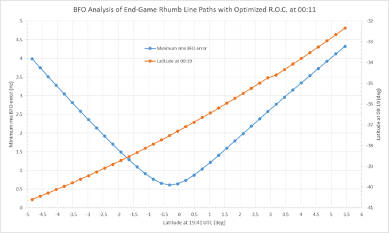
Figure 2: Rhumb line paths with optimized rate of descent at 00:11
indicating possible latitudes attained at 00:19.
(Note: R.O.C. means ‘Rate Of Climb’, which has negative values for a descent.)

 

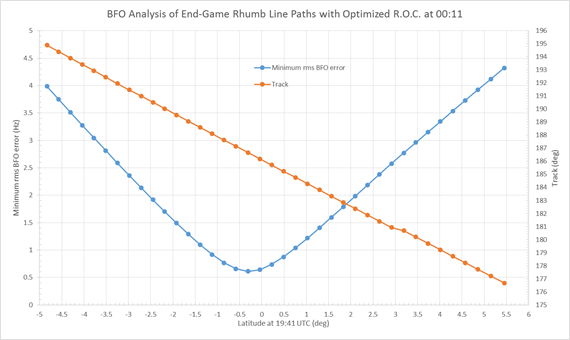
Figure 3: Rhumb line paths with optimized rate of descent at 00:11
indicating possible azimuths of such paths.

 

 

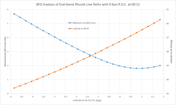
Figure 4: Rhumb line paths based on a constant altitude/no descent
at 00:11, indicating possible latitudes attained at 00:19.

 

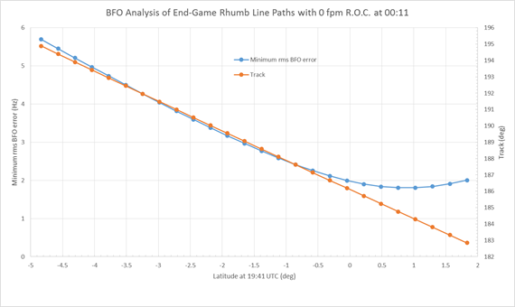
Figure 5: Rhumb line paths based on a constant altitude/no descent
at 00:11, indicating possible azimuths of such paths.

 

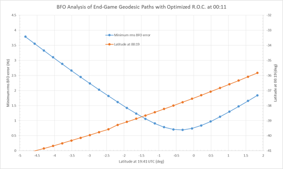
Figure 6: Geodesic paths based on an optimized rate of descent at 00:11
indicating possible latitudes attained at 00:19.

 

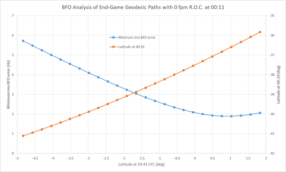
Figure 7: Geodesic paths, based on a constant altitude/no descent
at 00:11, indicating possible latitudes attained at 00:19.

 The most important points from the results shown in Figures 2 through 7 may be summarized as in Table 1:

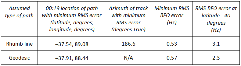
Table 1: Summary of results

Two interesting observations may be made concerning the optimum rhumb line path:

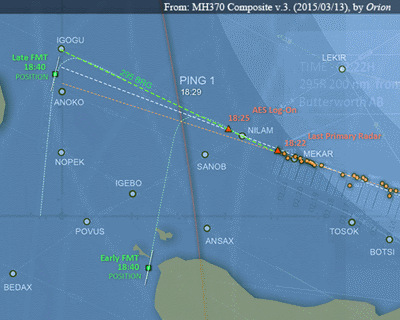
• If that path is extended back towards the north from 19:41, it passes close to waypoints ANOKO and IGOGU, as shown in Figure 8 below.
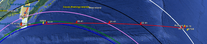
• Examining that path as it moves southwards on azimuth 186.6T, it is found to pass close to waypoint ISBIX, as shown in Figure 9 below.

A Skyvector plot of the overall optimum rhumb line path is available from here.

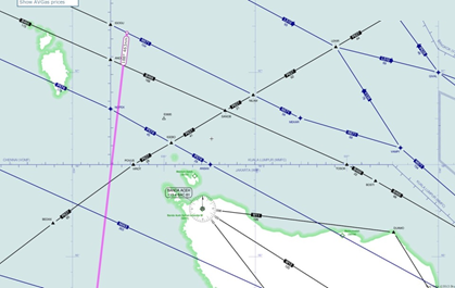
Figure 8: Propagating the optimum rhumb line flight path back northwards from 19:41.

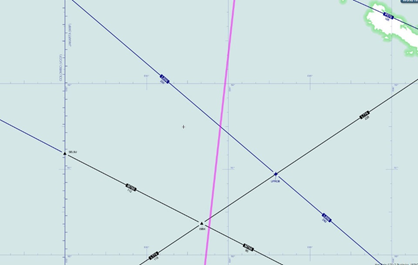
Figure 9: The optimum rhumb line flight path passes close to waypoint ISBIX.

 

5. Conclusions

The calculations presented here are based on a BFO error analysis assuming both (i) rhumb line/loxodrome; and (ii) great circle/geodesic paths, but without assuming any particular location and time of the final major turn. These calculations lead to a prediction of a set of likely flight paths and locations of the aircraft at 00:19, which have been ranked according to the RMS BFO error.

It is estimated that the path with the smallest RMS BFO error has a constant azimuth (i.e. is a rhumb line) of 186.6 degrees True; an end-point location (i.e. position at 00:19) that is near (-37.5, 89.0);  and a course that passes close to the three waypoints IGOGU, ANOKO and ISBIX.

The sensitivity of the RMS BFO error to changes in track and end-point location from the optimum solution appears to be quite low; consequently any location from latitude -34.5 to latitude -40.5 lying along the 7th ping arc cannot be ruled out based on BFO error analysis alone.  The search zone could possibly be reduced further by considering other factors such as aircraft performance. That is, this analysis has been based on DEO alone (allowing curved paths), with no CAD considerations involved (except for allowable paths being limited to rhumb lines or geodesics).

The analysis discussed herein could be further refined by considering the sensitivity to BTO errors, the fixed frequency bias utilized in the BFO analysis, and the rate of climb along the path (which has been assumed here to be zero – level flight – through until at least 00:11). This is beyond the scope of the current work, but preliminary studies suggest that the general conclusions reported here still hold.

Finally, it is to be emphasized that the analysis and results presented here are based on the standard interpretation of the BTO and BFO data. Assuming that the BTO and BFO data are reliable, the following Table 2 summarizes a compelling argument for a flight by an autopilot mode to the Southern Indian Ocean (SIO).

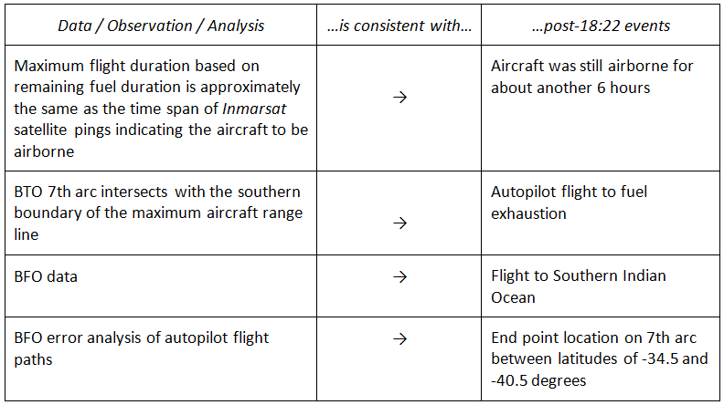
Table 2: Summary of arguments for an autopilot flight
to the Southern Indian Ocean.

6. Acknowledgements

I thank all members of the Independent Group (IG) for the active discussion and comments which have greatly helped me to understand much of the information that supports this analysis.

 

7. References

[1] ATSB (Australian Transport Safety Bureau) report (08 October 2014): Flight Path Analysis Update.

[2] ATSB (Australian Transport Safety Bureau) report (26 June 2014; updated 18 August 2014): MH370 – Definition of Underwater Search Areas. 

[3] Richard Godfrey (19 December 2014): MH370 Flight Path Model version 13.1. 

Deducing the Mid-Flight Speed of MH370

Brian Anderson 

2015 March 20

(Document prepared 26 December 2014)

 

1. Introduction 

Contact was lost with the crew of Malaysia Airlines flight MH370 at about 17:20 UTC on 7th March 2014. Despite extensive searches no trace has yet been found. Later in March 2014 the Inmarsat company released limited information regarding communications between MH370 and the Inmarsat-3F1 satellite, illustrating two hypothetical tracks southwards into the Indian Ocean, one at a constant speed of 400 knots, and one at 450 knots. A redacted version of the Inmarsat communication log was released at the end of May 2014. Specifically, the Burst Timing Offset (BTO) data released in the log file enabled a more accurate determination of the locations the so-called ‘ping rings’, and the distances of these rings from the sub-satellite position.

At about this time many other people, Inmarsat and the ATSB among them, made attempts to illustrate possible flight paths, choosing assumed speeds in order to intercept the ping rings at the appropriate times. It was very clear that the speed assumptions were not much more than guesses, and most flight paths required changes of aircraft heading at each ping ring in order to fit against the known travel times between those rings. Figures 1 and 2 illustrate some of these guesses; many other examples could be given.

Figure 1: An early example of putative paths to the Southern Indian Ocean using assumed speeds of 450 knots (yellow) and 400 knots (red).

Figure 2: An example of early priority search regions (since recognized to be incorrect). The intent in showing this example is to illustrate how various path models used changes of directions at the ping ring locations, which is obviously non-physical.  

The purpose of this paper is to show that it is possible to deduce the speed of MH370 in the mid-flight phase (specifically between about 19:41 and 20:41 UTC) using minimal data from the Inmarsat logs. The resulting value for the speed agrees well with the known speed of the aircraft soon after it had reached cruise altitude following take-off and before its turn back at 17:21 UTC near waypoint IGARI.

This hypothesis regarding how the aircraft speed might be deduced was first proposed in May 2014 (see below). The calculation was refined and updated progressively with new data over the following few weeks. This paper is a consolidation of a number of blog contributions during that period, in order to present the hypothesis in a concise fashion.

 

2. Initial observations

Before any BTO data were available, certain information was presented to a briefing of the Chinese families of MH370 passengers, at the Lido Hotel in Beijing, on about 28 April 2014. One of the slides presented became known as the ‘Fuzzy Chart of Elevation Angles’. This chart is shown below as Figure 3. Interestingly, the elevation angles (i.e. the apparent angular elevation of the satellite as seen from the aircraft; or, 90 degrees minus the zenith angle of the satellite as viewed from the aircraft) must have been derived from calculations based on the BTO data, but at this point no BTO data had been released publicly.

Figure 3: The Fuzzy Chart of Elevation Angles
derived from Inmarsat BTO values.

While this chart shows only a few data points it became the basis for various attempts at reverse-engineering the BTO data and thence the ping rings, and specifically the radii for these rings. At this time the Inmarsat definition for the BTO could be interpreted a number of different ways, and vigorous debate ensued amongst outside observers to determine the correct interpretation. Different interpretations resulted in radius variations of up to 50 NM (nautical miles).

In observing the elevation data points it is clear that the aircraft travelled away from the satellite immediately after take-off, then reversed its track and was coming closer to the satellite at least until about 19:40 UTC, then began moving away from the satellite again.

The reversal between 19:40 and 20:40 (approach to the satellite switching to recession)  is interesting in that there is clearly an instant between these two times when the aircraft was nearest to the satellite, and the elevation angle was therefore at a maximum. One can infer from this simple observation that at the point of closest approach the aircraft was therefore flying tangentially to the satellite.

From the fuzzy chart alone one could estimate the time of the closest approach at perhaps 12 minutes after 19:40. Work done by members of the Independent Group (IG) enabled the ping ring radii* at 19:40 and 20:40 to be estimated. An estimate of the elevation angle at the time of closest approach also enabled the calculation of the tangential radius. This was first suggested in a comment posted on May 16.

*In reality the ping rings or arcs are defined by equal ranges (as derived from the BTO values when they became available) from the satellite to the aircraft. Even if the aircraft were flying at a constant altitude (referred to either the WGS84 ellipsoid or Mean Sea Level, MSL) the ping rings would not truly be circular, because the Earth is not spherical. Regardless, using the term ‘radius’ to denote the sizes of the ping rings appears sensible, and for present purposes – estimating the aircraft’s speed averaged over an hour – the ping rings are indeed assumed to be arcs of circles.

 

3. Initial calculations

Armed with just three pieces of derived information – the estimated time of closest approach, and the radii of the 19:40 and 20:40 ping rings – it is possible to derive an estimate for the speed of the aircraft between these times (posted May 17; see also further comments posted on May 18 and May 20). One substantive assumption is necessary: that the aircraft was travelling in a straight line between these time, or nearly so. A slightly curved track would result in a greater distance being travelled, and hence a slightly greater speed being appropriate (than the lesser speed obtained from the method described here). Of course it is also necessary to assume a more-or-less constant speed between these times/between these ping rings.

Recognising that the geometry can be represented by two right-angled triangles, having a common/shared side (see Figure 4), planar geometry allows a solution for the length of the bases for these triangles to be determined, and hence the speed of the aircraft.

Figure 4: Geometry enabling the average aircraft speed between the
circa. 19:40 and circa. 20:20 pings to be estimated. 

Let:

r₁ = radius for the 19:40 ping ring

r₂ = radius for the 20:40 ping ring

r₀ = radius at the tangential point

t₁ = time interval from 19:40 to the tangential point occurrence (12 minutes)

t₂ = time interval from the tangential point occurrence to 20:40 (48 minutes)

d₁ = distance travelled from 19:40 to the tangential point

d₂ = distance travelled from the tangential point through to 20:40

v = the average speed of the aircraft between 19:40 and 20:40

Then:

d₁² = r₁² – r₀²

d₂² = r₂² – r₀²

d₁ = (t₁/60) * v

d₂ = (t₂/60) * v

(The division by 60 converts the time interval from minutes to fractions of an hour.)

Note that the radius to the tangential point (r₀) does not need to be known since it can be eliminated from the two equations above.

Rearranging:   v = √(r₂² _– r₁²) / ((t₂ /60)² – (t₁/60)²)

The initial values for r₁ and r₂ derived from the Fuzzy Chart were 1815 and 1852 NM respectively. Using these values and solving for v renders the aircraft speed as 476 knots.

This speed is significantly greater than most of the published guesses that were prevalent at the time.

A planar geometry solution to what is of course a spherical geometry situation is likely to result in a only a rough approximation, but the results were significant, and sufficiently encouraging to persist with the methodology while seeking accurate BTO data, an accurate satellite ephemeris, and solving the triangles using spherical geometry; as follows.

 

4. Better input data, more accuracy

A redacted Inmarsat communications log was released publicly towards the end of May 2014, providing a set of BTO values (delay times). By that time, ten weeks after loss of MH370, the correct interpretation of the Inmarsat BTO calculation had been established by Mike Exner [1], a member of the IG. This and the BTO data enabled a more accurate determination of the line-of-sight (LOS) range from the satellite to the aircraft, more precise timing for the ping ring intercepts, and an accurate calculation of the elevation angles first presented in the Fuzzy Chart (and then reverse-engineered to provide the satellite-aircraft ranges used earlier, as in section 3 above).

With new and reliable satellite ephemeris data it was also possible to perform accurate calculations for the ping ring radii from the correctly-timed sub-satellite position.

The speed deduction was improved by using these data and also a more-accurate estimation of the time of occurrence of the tangential point, using the minimum LOS L-Band transmission delay [1].

Figure 5 shows the calculated L-Band transmission delays for BTO data after 18:28 UTC.

Figure 5: The L-Band time delays for the aircraft-satellite link as a function of time during the flight of MH370.

 A third-order polynomial curve is fitted to the data points in Figure 5, leading to a solution:

Y = -0.0038x³ + 0.4433x² – 13.116x + 237.91

Differentiating this equation so as to determine the time of the minimum LOS range between the satellite and the aircraft:

dy/dx = -0.0114x² + 0.8866x – 13.116

When dy/dx = 0 one obtains

x = 19.870 (or 57.9015)

Converting this to a time, this yields an interval of 11.20 minutes after 19:41 UTC.

Note that it is by no means certain that the BTO for 18:28 UTC should fit conveniently on the smooth curve fitted to the LOS range delay. This might imply that the aircraft track from that time was more-or less a straight line, but there is no information to suggest that this is so.

In order to lessen the significance of that data point (at 18:28) a new nominal point was introduced at time 19:01.  A LOS range was determined for this point by fitting to the LOS range curve. It was hypothesised that turns which the aircraft may have made at around 18:28 to establish a track south would be well completed by 19:01, and hence this point ought to sit on the more-or-less straight track extending through 19:41 and 20:41. A nominal BTO figure was reverse-engineered for this nominal point.

With the new data it is also possible to calculate more accurate ping ring radii for the new precisely-determined times, 19:41:03 and 20:41:05 (as opposed to the approximate 19:40 and 20:40 read off the Fuzzy Chart), coupled with the accurate satellite ephemeris. Radii of 1757.25 and 1796.56 NM were used to solve once again the two right-angled triangles, but this time using spherical geometry.

Using the same nomenclature:

Let:

r₁ = radius for the 19:41 ping ring, expressed in radians

r₂ = radius for the 20:41 ping ring, expressed in radians

r₀ = radius at the tangential point, expressed in radians

t₁ = time after 19:41 that the tangential point occurs (11.2 minutes)

t₂ = time after the tangential point to 20:41 (48.8 minutes)

D = Great Circle distance travelled between 19:41 and 20:41

v = average speed of the aircraft between 19:41 and 20:41

Then:               cos(r₁) = cos(r₀) * cos(D * t₁/(t₁ + t₂))

and                  cos(r₂) = cos(r₀) * cos(D * t₂/(t₁ + t₂))

v = D/(t₁ + t₂)

The ground speed calculated by this method is now 494 knots.

The wind speed and direction for a potential southern track over this segment is about 21 knots from 65 degrees True [2]. Using this wind information, and the above ground speed of 494 knots on a track azimuth of 186 degrees, one can calculate the KTAS (True Air Speed, Knots) for the aircraft as being approximately 484 knots.

The fact that the KTAS matches the aircraft speed during cruise towards IGARI on the early portion of the flight adds a degree of confidence in this result, and provides a valuable basis for track and path estimates for later in the flight.

The astute may note that there is still an approximation (or implicit assumption) made in performing this calculation. This is due to the fact that the satellite is not stationary (although it is nearly so at about 19:41, having reached the apogee in its near-circular, 1.7-degree inclined orbit). This means that the apices of the right-angled triangles formed by the two ping radii and the tangent are not exactly coincidental. The error introduced by this assumption/approximation is small, and within the likely error margin from the estimated wind vectors for that location, and possible variations in ping ring radii from known BTO truncation and jitter. The range of sub-satellite positions is illustrated in Figure 6.

Figure 6: The movement of the sub-satellite position during the flight of MH370. In effect the method used in this paper assumes that the satellite remains in the same position between 19:41 and 20:41 UTC; the error caused by this necessary assumption is small.
Source: the above is Figure 8 in the paper published in the Journal of Navigation by Ashton et al. (2014).

5. Speed limits and observations

Since the speed obtained from this calculation is dependent upon the precise estimation of the time of the closest approach to the satellite (i.e. the tangent position), it is sensible to explore the possible limits of speed that might result from variations in this estimate.

It is sufficient to establish a maximum speed from published Boeing 777 performance data. A Mach number M=0.85 might be regarded as an upper limit, and this results in a KTAS of about 510 knots, depending on altitude and ambient temperature assumptions.

A special case exists when the tangent position occurs precisely at 19:41 (i.e. on the ping ring). In this case there is only one right-angled triangle to be solved. The ground speed derived for this case is 392 knots. For this occurrence to be true the LOS range from the satellite would have to exhibit its minimum precisely at 19:41. Examination of the numbers for LOS range, the BTO and the elevation angles suggest that this is not the case, and that the tangent point occurs after 19:41 (and well before 20:41).

One can therefore conclude that speeds less than 400 knots, or greater than 510 knots, are not plausible. It might also be reasonable to conclude that the aircraft was in fact close to the normally expected cruise speed, and also close to the normally expected cruise altitude of 35,000 ft.

In terms of aiding the overall understanding of the flight and therefore the speed of the aircraft it would be useful to know what autopilot Cost Index (CI) was programmed into the Flight Management Computer (FMC) for this flight. The IG has appealed several times for the CI used/programmed to be made available, but so far Malaysia Airlines has declined to do so. With such information in hand the IG would be able to refine its understanding of the constraints which can be placed on the flight: for example, knowing the CI would enable the likely speed(s) to be narrowed down, and knowing the fuel load the feasible flying range would be better defined and thus knowledge of the most-likely end-point refined.

References:

[1] Exner, M.L.: Deriving Net L-Band Propagation Delay and Range from BTO Values, 2014 May 28.

[2] Source for wind information is here.

Acknowledgements:

I thank everyone who assisted in discussions of this idea. This includes members of the IG, but also the various people who helped with their own comments and suggestions when I first proposed the concept.

This paper is available for download as a PDF (680 kB) from here.

Further Studies on the Path of MH370:
Turn Time and Final Azimuth

Sid Bennett and Geoff Hyman

2015 March 20 

 

The Independent Group (IG) operates by consensus and, for the present, there appears to be no compelling reason for the IG to issue a further statement regarding the probable final location of flight MH370. However, individuals and sub-groups have been pursuing details of the data and developing a better understanding of aspects of the event. This report is therefore one which is not intended as a statement by the IG as a whole, and is presented by the writers in order to further technical discussions relating to the likely location of the wreckage.

In particular, the focus of this report is on the flight path from the loss of primary radar contact at 18:22 to the last communication from the aircraft at 00:19 (2014 March 08; all times in this document are expressed in UTC). Details of the final descent are not addressed here.

Since the publication of the interim report by the Malaysian ICAO Annex 13 Safety Investigation team on 8^th March 2015, several studies have been produced that detail the flight path from takeoff to the loss of radar contact. An excerpt from an example published online by ‘Orion’ is shown as Figure 1 below.

Figure 1: Possible paths of MH370 across the Andaman Sea
according to ‘Orion’.

This portion of the path extends from a time before 18:22, where primary radar coverage existed, into the unknown flight regime thereafter. Consistent with the consensus that the BFO data require that the aircraft turn to the Southern Indian Ocean (SIO), two possible turns were illustrated. The early turn time leads to proposed end points well to the southwest of the current search area along the 7^th ping ring, while the turn at 18:40 is consistent with the previously-published IG end point.

The path simulation model (available from this website) used as the basis for the present report was developed by another IG member in response to specifications and recommendations made by the authors and others over the past year. The model simulates both geodesics and loxodromes on a modified WGS84 ellipsoid, and incorporates fuel burn prediction data, a meteorological reanalysis, an analytical solution for the BTO arc, and uses PAR5 satellite vectors (Henrik Rydberg: PAR5 Satellite Vectors for Inmarsat 3F1, based on ATSB vectors; see also this post), and various models for the Inmarsat SATCOM system. Simulated paths are scored by a cost function formulated by Geoff Hyman to quantify the errors in the fit of a single flight path to the combined BFO and BTO evidence. The cost function values enable the probabilities of competing flight path scenarios to be compared, even when the scenarios differ according to a range of different flight parameters.

A strong word of caution is needed here. Ordinarily a mathematical model is validated by testing it against data sets whose meaning is known. In this situation one would wish to use the model to analyze Inmarsat BTO/BFO data sets where the flight path characteristics are well-defined (i.e., routine flights). However, despite repeated requests by the IG for disclosure of such data, which is obviously available to the official investigators, no test set of data has been released. Consequently, one must treat the result as being the analysis of a single experiment without external validation.

Underlying the analysis presented here is the premise that, if the aircraft is to be found, the most probable location is that which can be deduced using a minimum number of arbitrary changes in flight parameters. This premise is, of course, debatable as there is a ‘margin of error’ associated with any specific path, including the most probable. The cost analysis also provides a means for assessing the width of this margin.

Consistent with this philosophy, the flight path is modeled as a loxodrome (rhumb line) having an origin at the last radar contact, making a single turn to the SIO and flying at a constant Mach number.

The predicted measurements of BFO and BTO are compared with the Inmarsat reported data and the combined error of the two measurements is used to optimize the modelled flight path.

An earlier version of this model was used to contribute to the IG recommended ‘end point’ location. That computation was a single path that exhibited the lowest ‘cost’, where ‘cost’ is a measure of the total BTO/BFO measurement error. Since that time, several proposed paths and end points have been proposed by other groups and individuals, and we have tried to understand the assumptions they have made and to compare their results with our work. The major difference between most models is related to the time at which the turn to the SIO is considered to have occurred.

The studies reported herein attempt to clarify this situation.  The first study is a determination of the most likely time for the turn to the SIO, which we call the FMT (final major turn), and the second study is an estimate of the probable azimuth range associated with the path subsequent to the turn, where the turn is presumed to have occurred at that most likely time. It should be stressed that paths with lower probability than the maximum probability still remain possibilities, but paths with very low probabilities might be eliminated.

First Study
The path from loss of radar contact at 18:22 is considered to continue at a constant Mach number and an azimuth of 295T until the turn time (i.e. the FMT). The turn time computation granularity was 30 seconds. In this context there are two events of note. At 18:25 the aircraft contacted the Inmarsat system and logged on, creating a sequence of data interchanges (BTO/BFO pairs), and at 18:40 there was an attempt to call the aircraft using the satellite system, which also created a sequence of data interchanges (BFO only).

As an overview of the results, it may be said that a turn to the SIO prior to 18:25 is inconsistent with the BFO at 18:25 because the approximate azimuth implied by the BFO value about near 295T. A turn to the south subsequent to 18:40 is similarly inconsistent with the BFO data at 18:40, which indicates an azimuth of about 192T (i.e. 12 degrees westwards of due south). The latter azimuth is not dissimilar to the final azimuth of approximately 186T that we deduce here, but is also consistent with an early turn occurring after 18:25 to an azimuth of 192T, which would result in the models proposed by other groups and individuals having an end point substantially to the southwest of the current search area (i.e. at latitudes well below 38S).

The results of the turn time study are shown in Figure 2, where the combined errors in the BFO and BTO are expressed as a ‘cost’.

Figure 2: The cost values (a numerical representation of the combined errors or deviations in the measured BTO and BFO values when compared to modelled aircraft flight paths southwards) as a function of the time of the Final Major Turn (FMT). 

Cost function values in excess of seven lead to very small probabilities and a turn at those times may  reasonably be rejected. Conversely, lower cost function values cannot reasonably be excluded. Figure 3 shows the relative probabilities of the FMT occurring at different times. It may be seen that there is a practical bound of 18:28 for the earliest turn time and of 18:40 for the latest turn time. These are well-determined, and attention might reasonably be confined to this range, at least for conditions resembling those adopted here. The strict bounds on the early and late turn times are seen to arise from the BFO measurements at 18:25 and 18:40. Simulations that begin at a later time, thus neglecting the period considered here, or which use the BTO data exclusively, will not exhibit these characteristics.

Figure 3: Relative probabilities for different times of occurrence of the final major turn (FMT).

Some of the alternative path models proposed by others use an early turn time. The probability per unit of time for turn time intervals preceding 18:34 is less than about one-third of the probability of turns occurring at or after the median turn time of 18:37; the most-likely individual time for the turn is 18:40 as it has the lowest cost.  This turn time is consistent with a FMT at waypoint IGOGU. We have not considered a turn time in the continuum between 18:25 and 18:37 as such turn times do not appear to be the basis of any proposed flight path models. However, another IG member has recently produced path solutions with the FMT occurring at 18:37 and examined a range of azimuths similar to those reported here. It is planned that these will be published in a separate report.

Second Study
Even if the turn is considered to occur at or very near 18:40, the final azimuth of the path is not certain. To explore this facet of the scenario, a series of paths was computed from a starting point at waypoint IGOGU with azimuths in 0.2 degree increments; relative probabilities for azimuths in this series are shown in Figure 4.

Figure 4: Relative probabilities for different azimuths of the path southwards following a final major turn assumed to take place at 18:40.

This result is consistent with the discrete ‘best path’ result of 186.4T which is discussed below. Extrapolating the path from IGOGU at this azimuth one finds that waypoint ISBIX is overflown. This may be a remarkable coincidence, or might be a consequence of a programmed flight path including IGOGU and ISBIX and continuing on a constant track thereafter. A constant track is one where the ground path of the flight path is at a constant azimuth, and that path does not vary with changing winds aloft.

Figure 5 shows an overview of the likely (i.e. lowest-cost) path of MH370 where the ping rings and times are shown for reference. Waypoints NILAM, IGOGU and ISBIX can be seen to define the early part of the path.

Figure 5: A likely path for MH370 to the Southern Indian Ocean based on our lowest-cost analysis of the BTO and BFO errors

Richard Godfrey’s latest end point at 37.47S, 89.28E , that of the ATSB (estimated centroid, courtesy Mike Exner, from quadrant A1 of Figure 4 in the ATSB report of 8th October 2014 ), and the IG’s ‘most probable’ end point of 37.71S, 88.75E, are also shown in more detail in Figure 6, where the green lines represent azimuths from the FMT of 184T and 188T, the red line is that for 186T, and the white line represents the 6^th ping ring.

Figure 6: Detail showing three possible end points near 37.6S, 89.0E. The green/red/green lines represent paths from the final major turn at 18:40 on azimuths of 188T, 186T and 184T. Yellow pins show estimated end points as discussed in the main text of this report. The point labelled
IG Sept 14 is that described in the report dated 26th September 2014.

 The differences in the end point estimates are not significant in the context of the current search area definition; however, one might consider the current search strategy to be inefficient if the most-likely end points are desired.

From a practical viewpoint, we conclude that MH370 most probably flew a path to the 7^th ping ring that is characterized by waypoints IGOGU and ISBIX and a continuation along a constant track. We have not considered any aspect of the final minutes of the flight as this is a subject being studied intensively by others, and will be covered in another report.

The views stated here are personal views and should therefore not be attributed to the IG as a whole, although it is supported by IG members. The information used is that which been made publicly-available from well-known sources and is accepted as valid for the purposes of this study. Having said this, we must express our gratitude to other members of the IG for sharing models and advising on matters of data analysis, communications, avionics and pilotage. We would be grateful if any errors were to be called to our attention.

This report is also available as a PDF download (432 kB) from here.