The Last 15 Minutes of Flight of MH370

Brian Anderson
Report prepared 2015 April 24

 

 Introduction

Determining what happened to MH370 during the last 15 minutes of flight is difficult, given the limited information available, yet it is important to arrive at some estimates of the aircraft altitude and path during this time. The path is needed in order to establish where the end point might be.

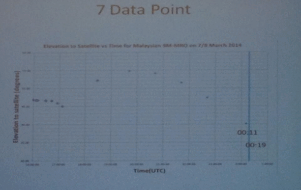
At the time of the Independent Group’s (IG) September 26 statement last year, the information available to help with the analysis of this period was limited to the satellite-derived BTO and BFO data at 00:11 and 00:19 UTC (on 2014 March 08), and the expectation that the engine failures with fuel exhaustion would not occur at precisely the same instant in time.

It was expected at that stage that knowledge of the engine Performance Degradation Allowance (PDA) figures would provide evidence as to which engine failed first, and also enable the remaining flight time before the second engine failed to be determined. Unfortunately the PDA information has not been made public by Malaysia Airlines.

The analysis of several simulation runs in a certified B777 level 4 simulator showed that knowing which engine fails first, and hence being able to determine the direction of the Thrust Asymmetry Compensation (TAC) deflection at the time of the second engine failure, is not a predictor of the flight characteristics of the aircraft following the second engine failure. Hence, knowing the PDAs is not immediately helpful in this regard (i.e. knowing which engine first ran out of fuel is not a necessity here). Rather, the flight characteristics, and in particular the propensity of the aircraft to bank into a turn immediately following the second engine failure, is a function of precisely how the aircraft was trimmed immediately before the first engine failure. The simulator trials showed that seconds after the second engine failure the TAC is reset to the cruise rudder trim position.

We know that each B777 aircraft is subtly different (as are most other aircraft) with respect to rudder trim in particular. One might say that they may be slightly ‘bent’ in terms of aerodynamics.  Some require a little left trim, some a little right, and some require neither in order to fly straight. In addition, individual pilots often adopt slightly different regimes in order to manage the trim (TAC) requirements. Without knowing how this particular aircraft handled historically – and even if we did know – it may not be possible to say with certainty if the aircraft would depart into a turn to the left or to the right following the second engine failure.

In performing the analysis presented in this paper I have made the following necessary assumptions:

• There was no manual intervention to control the aircraft during the last 15 minutes of flight;
• The aircraft was flying on autopilot during its passage south over the Indian Ocean until the second engine failure;
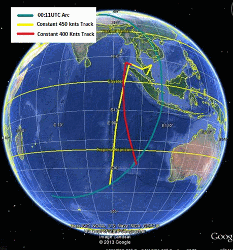
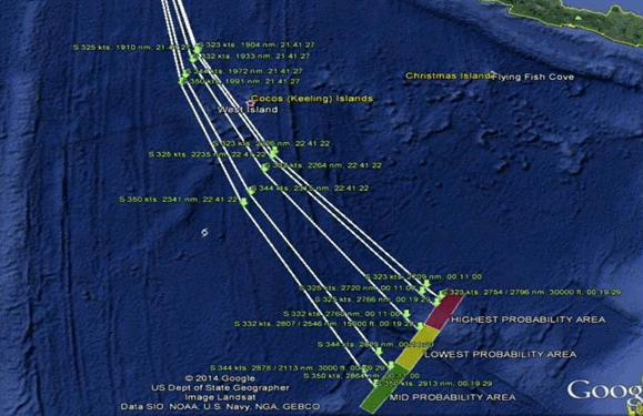
• The flight path is similar to the path discussed in the IG statement dated September 26 (and also a number of other independently-derived flight paths ending at similar latitudes, so that the precise flight path taken over the Indian Ocean is not significant here);
• The B777 level flight simulator runs previously studied by the IG (per Mike Exner) deliver a valid representation of how MH370 would be expected to have behaved near the end of its flight.

 

Fuel Data

With the release of the Factual Information statement by the Malaysian Safety Investigation Team on 08 March 2015 [reference 1], new information became available which enabled more analysis of the fuel consumption rates and better estimates of the engine failure timings, without requiring specific knowledge of the PDAs. This at least enables us to say with some certainty that it was the Right engine that failed (ran out of fuel) first.

When the first engine fails the TAC is immediately set to trim the aircraft to fly straight, and the auto-throttle increases thrust in order to maintain air speed and altitude, as far as possible.

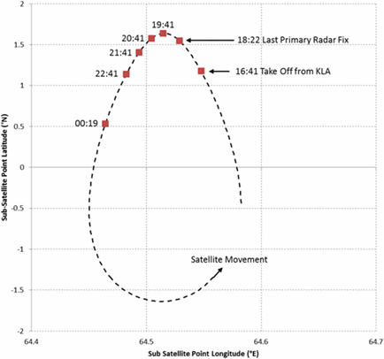
The ATSB, in its 26 June 2014 report [2], described the Satellite Data Unit (SDU) power up process and concluded that the 0019:29 log-on would have occurred three minutes and 40 seconds (+/- 10 seconds) following the second engine failure, and that the autopilot would have been disengaged for this period due to the interruption in electrical power. The SDU boot-up and final log-on is assumed to be a result of an automatic Auxiliary Power Unit (APU) start due to the loss of both electrical generators driven by the jet engines. The time required for the entire process, from loss of the second engine until the log-on, is 3m40s. This time was confirmed during the B777 flight simulator trials mentioned previously.

Note that the APU is supplied from the left main (fuel) manifold, and will continue to run only for as long as there is sufficient fuel in the fuel lines to the APU (given that the fuel tanks are empty, resulting in the jet engine failure). It is not surprising therefore that the final communication received from the aircraft was at 00:19:38, a possible cause being complete loss of power again, as the APU shut down. (An alternative explanation for the incomplete log-on might be mis-direction of the satellite communications antennae due to a spiral dive;  however the receiver power indications provided by Inmarsat [3] remain stable throughout all signal exchanges, and so this possibility seems less likely.)

The possibility that the aircraft impacted the sea at or very shortly after this time (00:19:38) should not be ignored: an implication of this would be that at that time the aircraft was at a low altitude, affecting the calculated position of the 7th/final ping arc, and therefore the search region for wreckage on the sea floor. Taking the aircraft altitude to be near zero at this time rather than at 35,000 feet has the effect of shifting the 7th ping arc by about 10 km to the northwest; this is discussed in more detail below.

A separate analysis of the fuel data is being undertaken within the IG [4] and it is sufficient to recognize here that the rate of fuel consumption rate for both engines combined for the remainder of the flight, from 17:07 through to 0019:29, is an average of about 6,072 kg/hr, (13,386 lbs/hr), and hence significantly lower than that shown for the take-off and climb phases of the flight as reported in the Factual Information [1], Appendix 1.6B. It is expected that the difference in fuel consumption rates between the two engines will be lower too (information in the Factual Information report indicates differences of 1.9 and 1.3 per cent, for take-off and climb: reference 4), and for the purpose of the ongoing discussion I have assumed, based on a simplified analysis, that this difference is 0.8 per cent. Using this figure it is possible to deduce that the Right engine failed close to, and perhaps a few seconds before, 00:11 UTC on 2014 March 08.

 

Flight path after the first engine failure

The simulator trials mentioned earlier illustrated clearly that following the first engine failure the auto-throttle increased thrust in the remaining engine, altitude was maintained, and the (longitudinal) pitch increased as the speed reduced so as to provide adequate lift. The deceleration observed was noted, and the Indicated Air Speeds (IAS) were converted to True Air Speeds in Knots (KTAS) for illustration in Figure 1, below. The observed trend is linear, with a deceleration of approximately 19 knots per minute. (dy/dx = -0.315 ´ 60 = -18.9). A deduction from this result is that the aircraft would still have been well above the best single engine speed and would have continued to fly at the same altitude for some minutes after the engine failure.

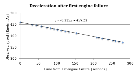
Figure 1: Deceleration after first engine failure

The flight dynamics are such that although drag and the available thrust are lower at higher altitude, the minimum drag speed also increases. Hence, coincident with one engine failing, we would expect deceleration to commence immediately and a reduction in altitude to begin as the minimum drag speed is approached. This was not observed in the simulator trials commencing at FL350 (Flight Level 350, nominally 35,000 feet but in actuality the geometric altitude depends on the atmospheric temperature and pressure). In fact the speed continued to decrease (below the minimum drag speed) without a descent being automatically commenced, but the ensuing part of the simulator trial was perforce cut short by the failure of the second engine. The speed (and time) at which MH370 would have begun to descend is therefore unknown from the simulator trial.

Turning back to what we know about the actual flight, the BFO at 00:11 suggests that at that instant the aircraft was descending at about 250 feet per minute. Together then, the BFO descent rate, the estimated time of the Right engine failure, and the simulator trials, may all be reconciled if the altitude was greater than FL350, in which case it is possible that a shallow descent commenced just prior to 00:11.

The appendices in the ATSB report [2] provide an indication of possible vertical descent rates resulting from loss-of-control events at high altitude. Descent rates of greater than 20,000 feet/min have been observed.

At the rate of speed (and altitude) reduction observed in the simulator trials, and because the aircraft is observed to be within a normally-expected flight envelope, it seems clear that the aircraft would still be close to FL350 (or higher) at the time the second/Left engine failed, at 00:15:49 (+/- 10 seconds). If, as a result of total loss of control at that time (autopilot failure due to interruption of electrical power) it happened that the aircraft impacted the sea at 00:19:38, the average descent rate would have been about 9,500 feet/min, which is well within the observations referenced in the preceding paragraph.

An immediate conclusion should be drawn at this point. Taking a conservative view (conservative, that is, in terms of the plausible distance travelled from the 6th ping arc at 00:11), the 7th arc position calculation should assume that the aircraft was at or near sea level (the surface of the reference ellipsoid) at time 00:19:38, and hence only a little above sea level at 00:19:29, and descending rapidly. At the latitudes of interest this will position the 7th arc at a distance of about 56 nm from the 00;11 arc along the 186 deg (from True North) azimuth in the vicinity of a latitude of 38 degrees South.

Assuming that the deceleration is a linear function, as observed in the simulator trials, the distance travelled from time 00:11 until the Left engine flames out can be calculated. For a range of speeds at 00:11, and assuming that at that time the aircraft was exactly on the 00:11/6th ping arc, the distances are illustrated in Figure 2, below.

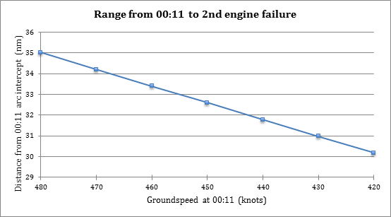
Figure 2: Distance travelled from 00:11 before second engine failure

Assuming a ground speed of 480 knots at 00:11 (equivalent to a wind-corrected KTAS of about 500 knots), and noting that this is likely to be an optimistic value since various IG path models suggest ground speeds between 429 and 455 knots at this point, and with a linear deceleration of 19 knots/minute, the ground speed at 00:15:49 would have been 389 knots, and the distance travelled from the 6th arc at 00:11 is 35nm (nautical miles). On an azimuth of 186 degT this will put the aircraft 21nm short of the 7th arc calculated at sea level for when the Left engine fails. Continuing with that rate of deceleration in a straight line (allowing for the effect of wind following the second engine failure), the total distance covered before 00:19:29 is 56 nm, which is just on the 7th arc calculated at sea level, but 6nm/10km short of the 7th arc at FL350.

 Continuing deceleration after the Left engine fails is not a certainty. It is possible that the speed may increase, since it is governed primarily by the relationship between the drag and the component of the aircraft weight acting down the flight path. With the assumption that there is no further deceleration after the Left engine fails, then in 3m 40s the distance covered is 24 nm and hence the aircraft is capable of reaching the 7th arc calculated at sea level, but still not capable of reaching the (FL350) 7th arc at 00:19:29, on the 186 degT azimuth.

As a comparison it is useful to test the outcome assuming a lower ground speed, say 429 knots (rather than 480 knots) at 00:11, and assuming the same rate of deceleration. In this case the ground speed at 00:15:49 would be down to 338 knots, and the distance travelled from the 6th arc at 00:11 would be only 31nm, which is 25nm short of the 7th arc calculated at sea level. In order to reach the 7th arc in a straight line on the same 186degT azimuth, a linear acceleration of approximately 50 knots per minute would be required, reaching a ground speed of 485 knots at 00:19:29. This seems unlikely, and indicates a likelihood that the speed at 00:11 was greater than 429 knots. Perhaps even more likely is the possibility that the aircraft turned towards the 7th arc at the time of the second engine failure.

 

Flight path after the second engine failure

Observations from the simulator trials suggests that following the failure of both engines the aircraft will bank into a turn almost immediately. The direction of the turn, and perhaps the rate of the initial turn, is a function of precisely how the aircraft was trimmed immediately before the first engine failure, and this is of course unknown. However, the observation that the aircraft may not be capable of reaching the 7th arc if that is assumed to be at 35,000 feet (as discussed above) may help in reaching a conclusion here.

For example, if the aircraft banked and turned to the right after the Left/second engine failed, then with the speed profile examined above, commencing at 480 knots at 00:11, it would not be possible to intercept the 7th arc until after 00:19:29, and even then the turn radius would have to be greater than about 48nm to intercept the arc at all.

Alternatively, if the aircraft banked and turned to the left after the Left/second engine failed then an intercept with the 7th arc at 00:19:29 is possible, but only if the turn radius is between 8 and 10 nm. At the assumed speed at which the turn commenced the required bank angle is approximately 15 degrees. Figure 3, below, illustrates these possibilities.

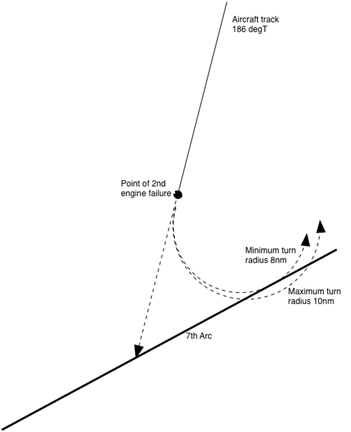
Figure 3: Illustrating possible tracks after second/Left engine failure

The simulator trials illustrate that after entering a banked turn, even one with a bank angle as shallow as 15 degrees, the aircraft does not recover to a wings-level attitude. Rather, over a period of about three minutes, and interspersed with possible phugoids, the bank angle will continue to increase until the aircraft enters a spiral dive. At that point the bank angle may have increased to 90 degrees, the aircraft may have rotated through three complete turns, the aircraft speed with respect to the air would exceed the normally-allowed maximum operating speed (VMO), but not necessarily have increased beyond maximum Mach operating speed (MMO) at that altitude so that it would likely not have suffered severe structural damage, and the descent rate would be up to 15,000 feet/minute. A high-speed uncontrolled impact with the sea would be inevitable.

Note that a descent rate of 15,000 feet/minute at the airspeeds of interest requires an aircraft track dipping only about 20 degrees below the horizon. More extreme descent rates are certainly possible.

 

Conclusions

Based on this analysis one may conclude that:

1. It is only with ground speeds greater than about 440 knots at 00:11 that it is possible subsequently to reach the 7th arc at sea level at all;
2. Following the Left/second engine failure, the aircraft very likely entered a turn to the left, a turn which developed into a spiral dive over the course of a few minutes resulting in a high speed impact inside the 7th arc as calculated for sea level.

It is clear from this analysis that establishing precisely where the 7th arc is located is very important from the point of view determining the path of the final few minutes of flight, and the underwater search strategy to be used. Based on the corrected BTO (18,400 microseconds) at 00:19:29 provided by the ATSB (2), the advisable position would be to establish the 7th arc at the surface of the reference ellipsoid (i.e., sea level) and not at high altitude (say 35,000 feet) the distinction between these shifting the 7th arc by about 6nm/10km.

 

Acknowledgements

 I thank members of the Independent Group (IG) for the active discussion, and contributions, which have greatly helped me to present this analysis and to arrive at the above conclusions. It is hoped that these will assist the official search teams in their identification of where to concentrate their efforts to achieve the highest likelihood of timely success.

 

References

[1]       Factual Information: Safety Investigation for MH370, published 08 March 2015, Malaysian ICAO Annex 13 Safety Investigation Team for MH370, Ministry of Transport, Malaysia.

[2]       MH370 – Definition of Underwater Search Areas, 26 June 2014 (updated 18 August), ATSB Transport Safety Report.

[3]       The Search for MH370, Journal of Navigation, September 2014, authors Chris Ashton, Alan Shuster Bruce, Gary Colledge and Mark Dickinson (Inmarsat).

[4]       Fuel Burn Analysis, spreadsheet by Mike Exner, April 2015. (Note that this link to Exner’s spreadsheet was added on 2015 June 20.)

 

 Autopilot Flight Path BFO Error Analysis

Yap Fook Fah

2015 March 24

(Updated 2015 April 20 to make the BTO and BFO Calculator available online: see reference [4] added at the very end.) 

A downloadable PDF of this report (867 kB) is available here.

1. Background

This report presents a Burst Frequency Offset (BFO) data error analysis of the end-game flight path of MH370 constrained by certain autopilot flight modes. The analysis is broadly similar in approach to that outlined in the ATSB reports [1, 2], but from which crucial quantitative results are not available for independent study.

Recall that the current search area is mainly defined by a compromise between two methods of analysis: “Constrained Autopilot Dynamics” (CAD), and “Data Error Optimisation” (DEO), as outlined in [1].

The CAD method assumes that the flight, at least after 18:40 UTC, was on some autopilot mode, and its range is limited by the amount of remaining fuel and aircraft performance. The ATSB report did not specify the time and location of the final major turn to the south. Further, the report did not provide details on how the generated paths were scored according to their “statistical consistency with the measured BFO and BTO values” [2].

In contrast, the DEO method does not take into account the flight mode, but simply seeks to rank a set of curved flight paths according to the deviation of the calculated BFO for each candidate flight path from the recorded values at the arc crossings after 18:40 UTC.

One problem is that the results from the two analyses are not quite consistent with each other. In particular, the DEO results imply that paths ending in the southern half of the CAD probability curve should be ranked much lower and be given less weight. In consequence, this has led to a compromise in the definition of the search area: “Area of interest on 0019 arc covers 80% of probable paths from the two analyses at 0011 …” [1]. This has the effect of shifting the search region further north than if only the CAD results were considered (see Figure 1 below).

Figure 1: Defining the search area (from reference [1]).

 

2. Objective

The objective of the present report is to reconstruct the end-game flight path BFO data error analysis with autopilot constraints, so as to obtain quantitative results for further evaluation and comparison with other types of analysis.

 

3. Methodology 

• A set of flight paths is generated starting from different locations on the 19:41 arc, each location being reachable from the last known radar position at 18:22 with the aircraft flying at feasible speeds.

• Each path is a rhumb line (or loxodrome) corresponding to a constant true track autopilot mode. The exercise is repeated assuming great circle paths (geodesics). The WGS84 model for the shape of the Earth is used.

• Each path is assumed to be flown at constant altitude. The exercise is repeated with an assumed rate of descent starting at 00:11 UTC (2014 March 08) that minimizes the BFO error.

• All paths cross the arcs at the recorded times, and therefore match the Burst Timing Offset (BTO) values exactly.

• The ground speed is allowed to vary. The speed profile is derived using a cubic polynomial function fitted over the five points at 19:41, 20:41, 21;41, 22:41 and 00:11. Integration of the speed over time gives the correct distance values at the arc crossings.

• A BFO fixed frequency bias of 150.26 Hz is used [3].

• The BFO values at the five arc crossings are calculated and compared to the recorded BFO values. The root-mean-square (RMS) error for each path is then calculated.

 

4. Results

Figures 2 through 5 are based on the paths southwards after 19:41 being rhumb lines (i.e. loxodromes), whereas Figures 6 and 7 are based on the modelled paths being great circles (i.e. geodesics).

Figure 2 shows, as a function of the assumed aircraft latitude at 19:41, (a) the variation of the minimum RMS BFO error; and (b) the latitude attained at 00:19, based on the rate of descent at 00:19 being optimized (i.e. the BFO value at that time being fitted).

Figure 3 is similar to Figure 2, but represents the azimuth of the derived rhumb line path from the position at 19:41.

Figures 4 and 5 are similar to Figures 2 and 3 except that they result from assuming no descent (a level flight) at 00:11.

Figure 6, for a great circle path as described above, is similar to Figure 2 in that the minimum RMS BFO error and the latitude attained at 00:19 is depicted, based on the rate of descent at 00:19 being optimized.

Figure 7 is similar to Figure 3: the minimum RMS BFO error and the latitude attained at 00:19 is depicted, based on no descent (a level flight) at 00:11.

Obviously there are no graphs/figures for constant azimuths in the case of these great circle (geodesic) paths because such paths have constantly-changing azimuths.

Figure 2: Rhumb line paths with optimized rate of descent at 00:11
indicating possible latitudes attained at 00:19.
(Note: R.O.C. means ‘Rate Of Climb’, which has negative values for a descent.)

 

Figure 3: Rhumb line paths with optimized rate of descent at 00:11
indicating possible azimuths of such paths.

 

 

Figure 4: Rhumb line paths based on a constant altitude/no descent
at 00:11, indicating possible latitudes attained at 00:19.

 

Figure 5: Rhumb line paths based on a constant altitude/no descent
at 00:11, indicating possible azimuths of such paths.

 

Figure 6: Geodesic paths based on an optimized rate of descent at 00:11
indicating possible latitudes attained at 00:19.

 

Figure 7: Geodesic paths, based on a constant altitude/no descent
at 00:11, indicating possible latitudes attained at 00:19.

 The most important points from the results shown in Figures 2 through 7 may be summarized as in Table 1:

Table 1: Summary of results

Two interesting observations may be made concerning the optimum rhumb line path:

• If that path is extended back towards the north from 19:41, it passes close to waypoints ANOKO and IGOGU, as shown in Figure 8 below.
• Examining that path as it moves southwards on azimuth 186.6T, it is found to pass close to waypoint ISBIX, as shown in Figure 9 below.

A Skyvector plot of the overall optimum rhumb line path is available from here.

Figure 8: Propagating the optimum rhumb line flight path back northwards from 19:41.

Figure 9: The optimum rhumb line flight path passes close to waypoint ISBIX.

 

5. Conclusions

The calculations presented here are based on a BFO error analysis assuming both (i) rhumb line/loxodrome; and (ii) great circle/geodesic paths, but without assuming any particular location and time of the final major turn. These calculations lead to a prediction of a set of likely flight paths and locations of the aircraft at 00:19, which have been ranked according to the RMS BFO error.

It is estimated that the path with the smallest RMS BFO error has a constant azimuth (i.e. is a rhumb line) of 186.6 degrees True; an end-point location (i.e. position at 00:19) that is near (-37.5, 89.0);  and a course that passes close to the three waypoints IGOGU, ANOKO and ISBIX.

The sensitivity of the RMS BFO error to changes in track and end-point location from the optimum solution appears to be quite low; consequently any location from latitude -34.5 to latitude -40.5 lying along the 7th ping arc cannot be ruled out based on BFO error analysis alone.  The search zone could possibly be reduced further by considering other factors such as aircraft performance. That is, this analysis has been based on DEO alone (allowing curved paths), with no CAD considerations involved (except for allowable paths being limited to rhumb lines or geodesics).

The analysis discussed herein could be further refined by considering the sensitivity to BTO errors, the fixed frequency bias utilized in the BFO analysis, and the rate of climb along the path (which has been assumed here to be zero – level flight – through until at least 00:11). This is beyond the scope of the current work, but preliminary studies suggest that the general conclusions reported here still hold.

Finally, it is to be emphasized that the analysis and results presented here are based on the standard interpretation of the BTO and BFO data. Assuming that the BTO and BFO data are reliable, the following Table 2 summarizes a compelling argument for a flight by an autopilot mode to the Southern Indian Ocean (SIO).

Table 2: Summary of arguments for an autopilot flight
to the Southern Indian Ocean.

6. Acknowledgements

I thank all members of the Independent Group (IG) for the active discussion and comments which have greatly helped me to understand much of the information that supports this analysis.

 

7. References

[1] ATSB (Australian Transport Safety Bureau) report (08 October 2014): Flight Path Analysis Update.

[2] ATSB (Australian Transport Safety Bureau) report (26 June 2014; updated 18 August 2014): MH370 – Definition of Underwater Search Areas. 

[3] Richard Godfrey (19 December 2014): MH370 Flight Path Model version 13.1. 

Deducing the Mid-Flight Speed of MH370

Brian Anderson 

2015 March 20

(Document prepared 26 December 2014)

 

1. Introduction 

Contact was lost with the crew of Malaysia Airlines flight MH370 at about 17:20 UTC on 7th March 2014. Despite extensive searches no trace has yet been found. Later in March 2014 the Inmarsat company released limited information regarding communications between MH370 and the Inmarsat-3F1 satellite, illustrating two hypothetical tracks southwards into the Indian Ocean, one at a constant speed of 400 knots, and one at 450 knots. A redacted version of the Inmarsat communication log was released at the end of May 2014. Specifically, the Burst Timing Offset (BTO) data released in the log file enabled a more accurate determination of the locations the so-called ‘ping rings’, and the distances of these rings from the sub-satellite position.

At about this time many other people, Inmarsat and the ATSB among them, made attempts to illustrate possible flight paths, choosing assumed speeds in order to intercept the ping rings at the appropriate times. It was very clear that the speed assumptions were not much more than guesses, and most flight paths required changes of aircraft heading at each ping ring in order to fit against the known travel times between those rings. Figures 1 and 2 illustrate some of these guesses; many other examples could be given.

Figure 1: An early example of putative paths to the Southern Indian Ocean using assumed speeds of 450 knots (yellow) and 400 knots (red).

Figure 2: An example of early priority search regions (since recognized to be incorrect). The intent in showing this example is to illustrate how various path models used changes of directions at the ping ring locations, which is obviously non-physical.  

The purpose of this paper is to show that it is possible to deduce the speed of MH370 in the mid-flight phase (specifically between about 19:41 and 20:41 UTC) using minimal data from the Inmarsat logs. The resulting value for the speed agrees well with the known speed of the aircraft soon after it had reached cruise altitude following take-off and before its turn back at 17:21 UTC near waypoint IGARI.

This hypothesis regarding how the aircraft speed might be deduced was first proposed in May 2014 (see below). The calculation was refined and updated progressively with new data over the following few weeks. This paper is a consolidation of a number of blog contributions during that period, in order to present the hypothesis in a concise fashion.

 

2. Initial observations

Before any BTO data were available, certain information was presented to a briefing of the Chinese families of MH370 passengers, at the Lido Hotel in Beijing, on about 28 April 2014. One of the slides presented became known as the ‘Fuzzy Chart of Elevation Angles’. This chart is shown below as Figure 3. Interestingly, the elevation angles (i.e. the apparent angular elevation of the satellite as seen from the aircraft; or, 90 degrees minus the zenith angle of the satellite as viewed from the aircraft) must have been derived from calculations based on the BTO data, but at this point no BTO data had been released publicly.

Figure 3: The Fuzzy Chart of Elevation Angles
derived from Inmarsat BTO values.

While this chart shows only a few data points it became the basis for various attempts at reverse-engineering the BTO data and thence the ping rings, and specifically the radii for these rings. At this time the Inmarsat definition for the BTO could be interpreted a number of different ways, and vigorous debate ensued amongst outside observers to determine the correct interpretation. Different interpretations resulted in radius variations of up to 50 NM (nautical miles).

In observing the elevation data points it is clear that the aircraft travelled away from the satellite immediately after take-off, then reversed its track and was coming closer to the satellite at least until about 19:40 UTC, then began moving away from the satellite again.

The reversal between 19:40 and 20:40 (approach to the satellite switching to recession)  is interesting in that there is clearly an instant between these two times when the aircraft was nearest to the satellite, and the elevation angle was therefore at a maximum. One can infer from this simple observation that at the point of closest approach the aircraft was therefore flying tangentially to the satellite.

From the fuzzy chart alone one could estimate the time of the closest approach at perhaps 12 minutes after 19:40. Work done by members of the Independent Group (IG) enabled the ping ring radii* at 19:40 and 20:40 to be estimated. An estimate of the elevation angle at the time of closest approach also enabled the calculation of the tangential radius. This was first suggested in a comment posted on May 16.

*In reality the ping rings or arcs are defined by equal ranges (as derived from the BTO values when they became available) from the satellite to the aircraft. Even if the aircraft were flying at a constant altitude (referred to either the WGS84 ellipsoid or Mean Sea Level, MSL) the ping rings would not truly be circular, because the Earth is not spherical. Regardless, using the term ‘radius’ to denote the sizes of the ping rings appears sensible, and for present purposes – estimating the aircraft’s speed averaged over an hour – the ping rings are indeed assumed to be arcs of circles.

 

3. Initial calculations

Armed with just three pieces of derived information – the estimated time of closest approach, and the radii of the 19:40 and 20:40 ping rings – it is possible to derive an estimate for the speed of the aircraft between these times (posted May 17; see also further comments posted on May 18 and May 20). One substantive assumption is necessary: that the aircraft was travelling in a straight line between these time, or nearly so. A slightly curved track would result in a greater distance being travelled, and hence a slightly greater speed being appropriate (than the lesser speed obtained from the method described here). Of course it is also necessary to assume a more-or-less constant speed between these times/between these ping rings.

Recognising that the geometry can be represented by two right-angled triangles, having a common/shared side (see Figure 4), planar geometry allows a solution for the length of the bases for these triangles to be determined, and hence the speed of the aircraft.

Figure 4: Geometry enabling the average aircraft speed between the
circa. 19:40 and circa. 20:20 pings to be estimated. 

Let:

r₁ = radius for the 19:40 ping ring

r₂ = radius for the 20:40 ping ring

r₀ = radius at the tangential point

t₁ = time interval from 19:40 to the tangential point occurrence (12 minutes)

t₂ = time interval from the tangential point occurrence to 20:40 (48 minutes)

d₁ = distance travelled from 19:40 to the tangential point

d₂ = distance travelled from the tangential point through to 20:40

v = the average speed of the aircraft between 19:40 and 20:40

Then:

d₁² = r₁² – r₀²

d₂² = r₂² – r₀²

d₁ = (t₁/60) * v

d₂ = (t₂/60) * v

(The division by 60 converts the time interval from minutes to fractions of an hour.)

Note that the radius to the tangential point (r₀) does not need to be known since it can be eliminated from the two equations above.

Rearranging:   v = √(r₂² _– r₁²) / ((t₂ /60)² – (t₁/60)²)

The initial values for r₁ and r₂ derived from the Fuzzy Chart were 1815 and 1852 NM respectively. Using these values and solving for v renders the aircraft speed as 476 knots.

This speed is significantly greater than most of the published guesses that were prevalent at the time.

A planar geometry solution to what is of course a spherical geometry situation is likely to result in a only a rough approximation, but the results were significant, and sufficiently encouraging to persist with the methodology while seeking accurate BTO data, an accurate satellite ephemeris, and solving the triangles using spherical geometry; as follows.

 

4. Better input data, more accuracy

A redacted Inmarsat communications log was released publicly towards the end of May 2014, providing a set of BTO values (delay times). By that time, ten weeks after loss of MH370, the correct interpretation of the Inmarsat BTO calculation had been established by Mike Exner [1], a member of the IG. This and the BTO data enabled a more accurate determination of the line-of-sight (LOS) range from the satellite to the aircraft, more precise timing for the ping ring intercepts, and an accurate calculation of the elevation angles first presented in the Fuzzy Chart (and then reverse-engineered to provide the satellite-aircraft ranges used earlier, as in section 3 above).

With new and reliable satellite ephemeris data it was also possible to perform accurate calculations for the ping ring radii from the correctly-timed sub-satellite position.

The speed deduction was improved by using these data and also a more-accurate estimation of the time of occurrence of the tangential point, using the minimum LOS L-Band transmission delay [1].

Figure 5 shows the calculated L-Band transmission delays for BTO data after 18:28 UTC.

Figure 5: The L-Band time delays for the aircraft-satellite link as a function of time during the flight of MH370.

 A third-order polynomial curve is fitted to the data points in Figure 5, leading to a solution:

Y = -0.0038x³ + 0.4433x² – 13.116x + 237.91

Differentiating this equation so as to determine the time of the minimum LOS range between the satellite and the aircraft:

dy/dx = -0.0114x² + 0.8866x – 13.116

When dy/dx = 0 one obtains

x = 19.870 (or 57.9015)

Converting this to a time, this yields an interval of 11.20 minutes after 19:41 UTC.

Note that it is by no means certain that the BTO for 18:28 UTC should fit conveniently on the smooth curve fitted to the LOS range delay. This might imply that the aircraft track from that time was more-or less a straight line, but there is no information to suggest that this is so.

In order to lessen the significance of that data point (at 18:28) a new nominal point was introduced at time 19:01.  A LOS range was determined for this point by fitting to the LOS range curve. It was hypothesised that turns which the aircraft may have made at around 18:28 to establish a track south would be well completed by 19:01, and hence this point ought to sit on the more-or-less straight track extending through 19:41 and 20:41. A nominal BTO figure was reverse-engineered for this nominal point.

With the new data it is also possible to calculate more accurate ping ring radii for the new precisely-determined times, 19:41:03 and 20:41:05 (as opposed to the approximate 19:40 and 20:40 read off the Fuzzy Chart), coupled with the accurate satellite ephemeris. Radii of 1757.25 and 1796.56 NM were used to solve once again the two right-angled triangles, but this time using spherical geometry.

Using the same nomenclature:

Let:

r₁ = radius for the 19:41 ping ring, expressed in radians

r₂ = radius for the 20:41 ping ring, expressed in radians

r₀ = radius at the tangential point, expressed in radians

t₁ = time after 19:41 that the tangential point occurs (11.2 minutes)

t₂ = time after the tangential point to 20:41 (48.8 minutes)

D = Great Circle distance travelled between 19:41 and 20:41

v = average speed of the aircraft between 19:41 and 20:41

Then:               cos(r₁) = cos(r₀) * cos(D * t₁/(t₁ + t₂))

and                  cos(r₂) = cos(r₀) * cos(D * t₂/(t₁ + t₂))

v = D/(t₁ + t₂)

The ground speed calculated by this method is now 494 knots.

The wind speed and direction for a potential southern track over this segment is about 21 knots from 65 degrees True [2]. Using this wind information, and the above ground speed of 494 knots on a track azimuth of 186 degrees, one can calculate the KTAS (True Air Speed, Knots) for the aircraft as being approximately 484 knots.

The fact that the KTAS matches the aircraft speed during cruise towards IGARI on the early portion of the flight adds a degree of confidence in this result, and provides a valuable basis for track and path estimates for later in the flight.

The astute may note that there is still an approximation (or implicit assumption) made in performing this calculation. This is due to the fact that the satellite is not stationary (although it is nearly so at about 19:41, having reached the apogee in its near-circular, 1.7-degree inclined orbit). This means that the apices of the right-angled triangles formed by the two ping radii and the tangent are not exactly coincidental. The error introduced by this assumption/approximation is small, and within the likely error margin from the estimated wind vectors for that location, and possible variations in ping ring radii from known BTO truncation and jitter. The range of sub-satellite positions is illustrated in Figure 6.

Figure 6: The movement of the sub-satellite position during the flight of MH370. In effect the method used in this paper assumes that the satellite remains in the same position between 19:41 and 20:41 UTC; the error caused by this necessary assumption is small.
Source: the above is Figure 8 in the paper published in the Journal of Navigation by Ashton et al. (2014).

5. Speed limits and observations

Since the speed obtained from this calculation is dependent upon the precise estimation of the time of the closest approach to the satellite (i.e. the tangent position), it is sensible to explore the possible limits of speed that might result from variations in this estimate.

It is sufficient to establish a maximum speed from published Boeing 777 performance data. A Mach number M=0.85 might be regarded as an upper limit, and this results in a KTAS of about 510 knots, depending on altitude and ambient temperature assumptions.

A special case exists when the tangent position occurs precisely at 19:41 (i.e. on the ping ring). In this case there is only one right-angled triangle to be solved. The ground speed derived for this case is 392 knots. For this occurrence to be true the LOS range from the satellite would have to exhibit its minimum precisely at 19:41. Examination of the numbers for LOS range, the BTO and the elevation angles suggest that this is not the case, and that the tangent point occurs after 19:41 (and well before 20:41).

One can therefore conclude that speeds less than 400 knots, or greater than 510 knots, are not plausible. It might also be reasonable to conclude that the aircraft was in fact close to the normally expected cruise speed, and also close to the normally expected cruise altitude of 35,000 ft.

In terms of aiding the overall understanding of the flight and therefore the speed of the aircraft it would be useful to know what autopilot Cost Index (CI) was programmed into the Flight Management Computer (FMC) for this flight. The IG has appealed several times for the CI used/programmed to be made available, but so far Malaysia Airlines has declined to do so. With such information in hand the IG would be able to refine its understanding of the constraints which can be placed on the flight: for example, knowing the CI would enable the likely speed(s) to be narrowed down, and knowing the fuel load the feasible flying range would be better defined and thus knowledge of the most-likely end-point refined.

References:

[1] Exner, M.L.: Deriving Net L-Band Propagation Delay and Range from BTO Values, 2014 May 28.

[2] Source for wind information is here.

Acknowledgements:

I thank everyone who assisted in discussions of this idea. This includes members of the IG, but also the various people who helped with their own comments and suggestions when I first proposed the concept.

This paper is available for download as a PDF (680 kB) from here.