The Orbital Debris Collision Hazard for
Satellites in Geostationary Orbit

Duncan Steel
2015 April 29

Introduction

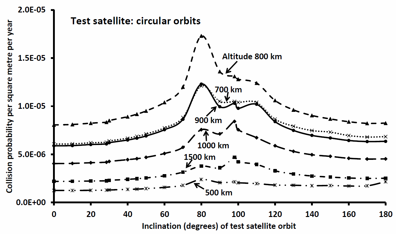
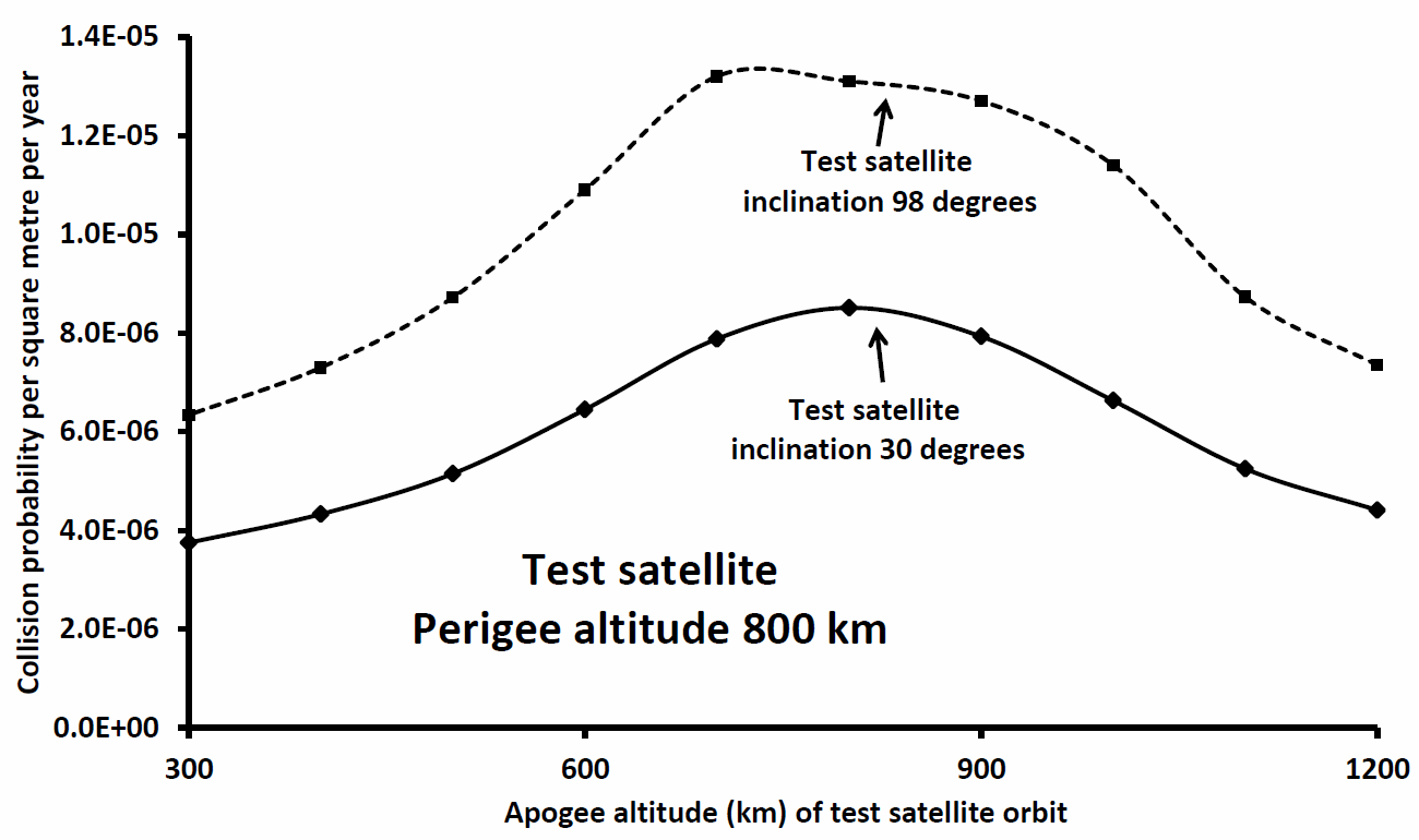
In my two previous posts (here, and here) regarding the orbital debris collision hazard I have been considering only test satellites in low-Earth orbit (LEO). In this post I turn my attention to satellites in geostationary orbit (GEO); that is, satellites in orbits that have periods of one sidereal day (i.e. altitudes near 35,800 km) and are in near-circular (i.e. low eccentricity) paths close to the equatorial plane (i.e. low inclination). Such orbits are used for many communications satellites, and are sometimes termed Clarke orbits.

 

A crude estimation of the typical collision probability in GEO

In principle it is straightforward to derive an estimate of the collision probability with space debris for a satellite in GEO. Consider the diagram below. The white circle shows the orbit of a geostationary communications satellite: there are many such satellites in GEO, but they remain in set positions due to their operators performing station-keeping burns/manoeuvres and so cannot collide with each other. Even a GEO satellite which is no longer under control only has a small drift speed (much smaller than the GEO orbital speed of  3.075 km/sec) and so the risk of inter-satellite collisions is very small, if we are considering only true geostationary satellites.

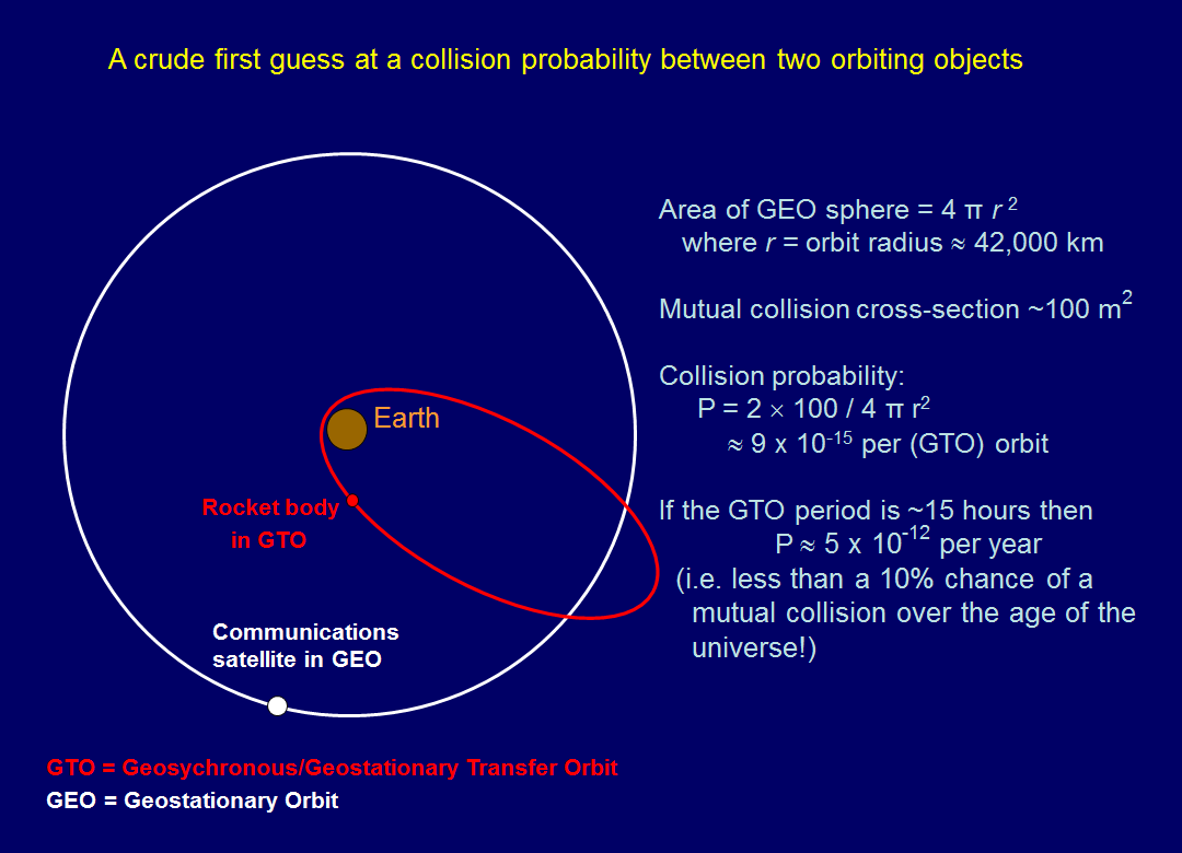
This is not true, however, for orbiting objects that cross the GEO altitude. The red ellipse in the diagram is intended to represent a rocket body in a geostationary/geosynchronous transfer orbit, having performed its purpose in carrying a GEO satellite to the necessary altitude. That defunct rocket body will pose a collision hazard to all functioning satellites in the geostationary band, as its argument of perigee and longitude of the node precess under gravitational perturbations due to the Moon and the Sun, and also the Earth’s oblateness (dependent upon the altitude of its perigee).

Imagine a sphere with radius (r) equal to the distance of the geostationary band from the centre of the Earth (about 42,000 km). That sphere has an area of 4πr². The rocket body, having an apogee above the geostationary band as shown, crosses that band twice per orbit, giving it two chances to hit that one particular communications satellite. If we estimate the mutual collision cross-section to be 100 square metres, then the probability of a collision is given by 2 × 100 / 4πr² which is a shade less than one part in 10¹⁴ per orbit of the GTO object (the rocket body). That GTO will have a period lower than one sidereal day, perhaps about 15 hours, or one part in 584 of a year, so that our estimate of the mutual collision probability becomes about 5 or 6 × 10^-12 per year.

To put that figure into some perspective, the universe is about 13.8 billion years old, and so a mutual collision would have a probability of occurrence of less than ten per cent over such a timescale. (Of course, the solar system is only about one-third the age of the universe; and over such phenomenal timescales all manner of other things happen.)

This, however, was a calculation for a mutual collision between only one pair of orbiting objects. The reality is that there are hundreds of satellites in geostationary orbit; and hundreds of rocket bodies and fuel tanks and other debris items crossing the GEO altitude, so that a more sophisticated assessment of the collision hazard is warranted.

 

Specific example orbits

The Inmarsat 5F2 communications satellite was launched on 2015 February 01 and inserted into geostationary orbit. The Briz-M rocket booster that was used to carry it to its final altitude remains in a GTO similar to that shown in the preceding diagram. Orbital parameters for the two objects in question are shown in the table below; note that the inclination and eccentricity of Inmarsat-5F2 in particular will vary from day-to-day and week-to-week under the influence of gravitational (and radiation-induced) perturbations, plus station-keeping burns by the operating company.

Name	International Designator	Satellite Catalogue Number (SCN)	Perigee altitude (km)	Apogee altitude (km)	Eccentricity	Inclination to the Equator (degrees)
Inmarsat-5F2	2015-005A	40384	35,551	36,029	0.000165	0.0338
Inmarsat-5F2 Rocket Body	2015-005B	40385	2,775	63,223	0.767648	27.6213
Inmarsat-5F2 Fuel Tank	2015-005C	40386	355	14,849	0.518453	50.7385

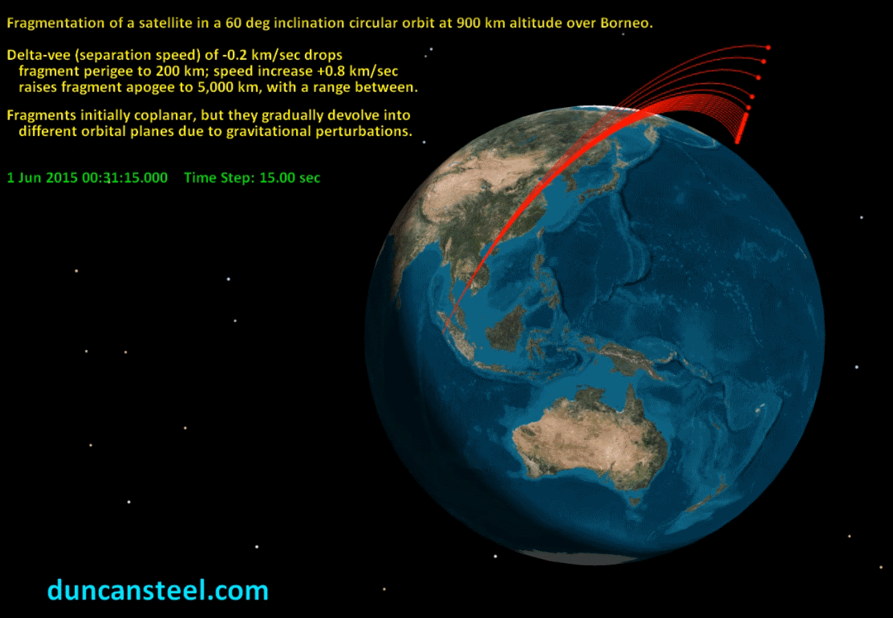
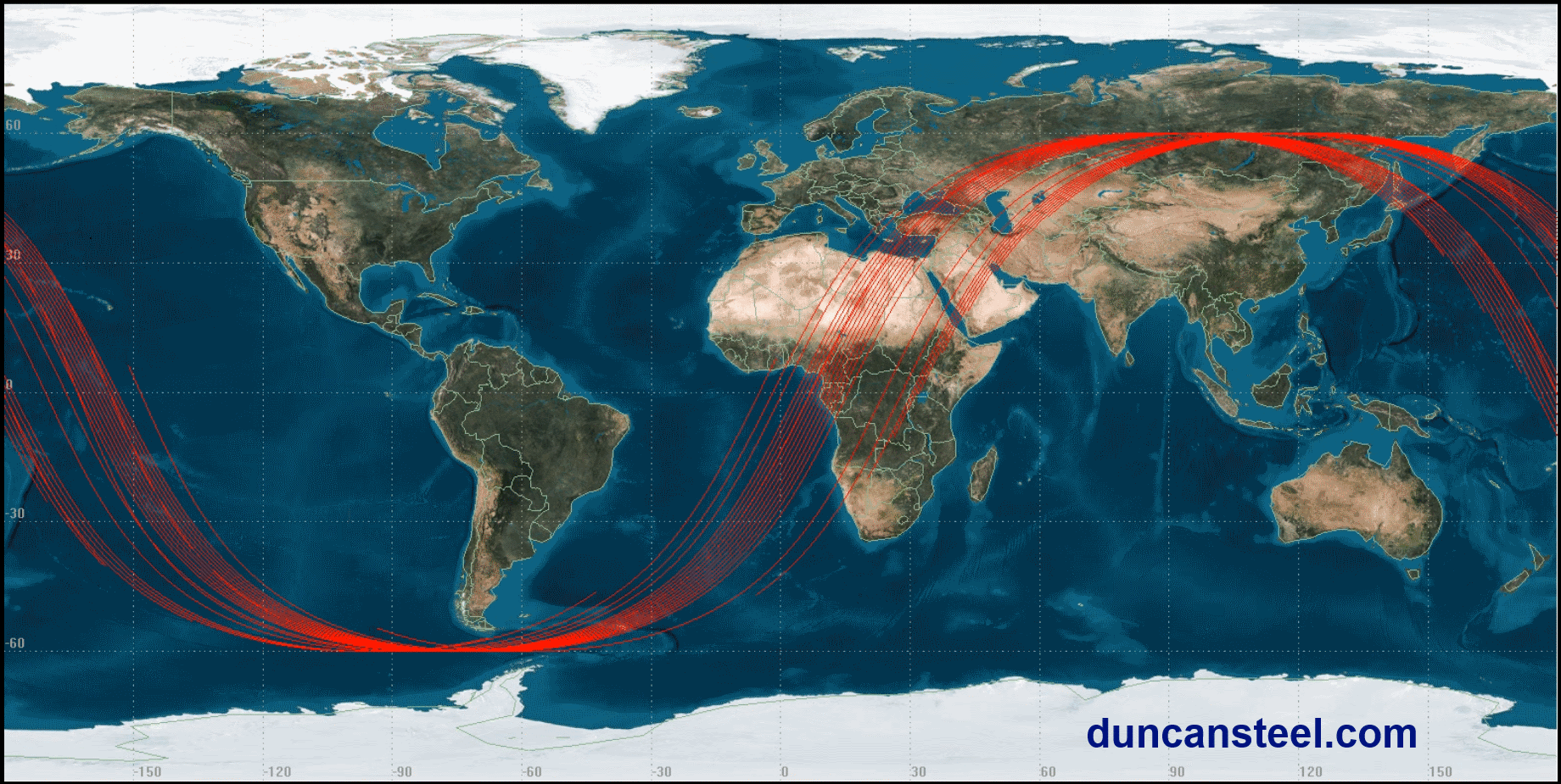
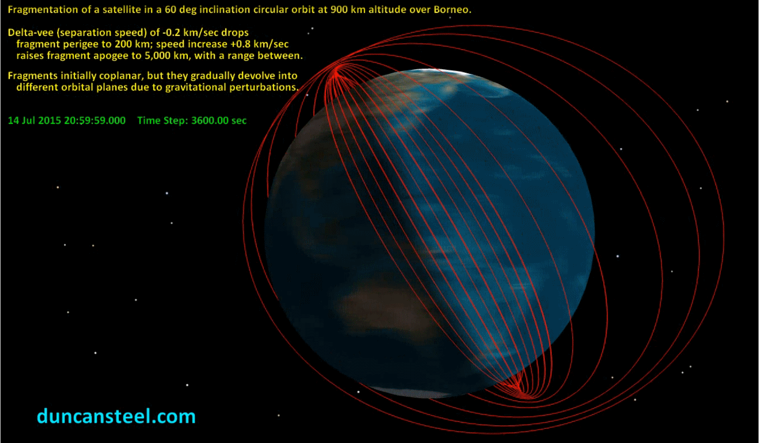
The final line in the table, for the fuel tank left in a lower orbit, plays no further part in the present calculations and is included simply for completeness. The orbits of the first two objects are shown in the graphic below, with three views being given so as to indicate the three-dimensional nature of the geometry. In addition a short movie portraying the movements of the two objects over five days is available for viewing and download from here (1.44MB).

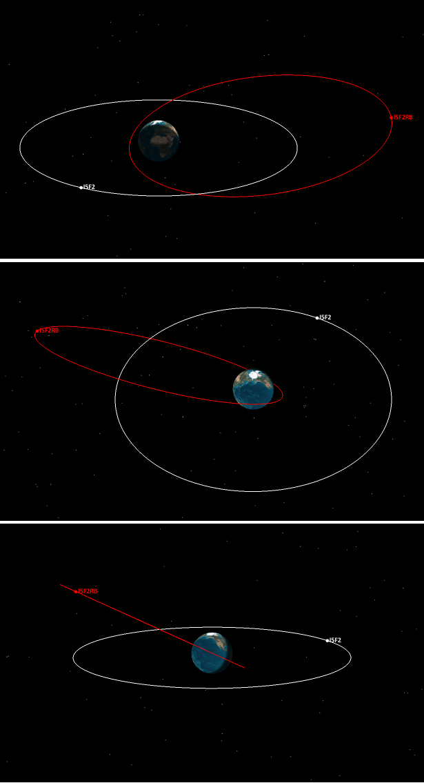
Graphic above: The orbits of the Inmarsat-5F2 satellite (in a near-circular geostationary orbit) and also the rocket body that carried it there, that rocket body (labelled I5F2RB above) having been left in an orbit with eccentricity near 0.77 and a perigee altitude of a few thousand kilometres. 

Using the orbital parameters listed above I can now calculate the separate collision probabilities involving (a) Inmarsat-5F2 itself; and (b) the Briz-M rocket body used to carry Inmarsat-5F2 to its geostationary orbit, against all objects in the tracked orbiting object catalogue. In a previous post I described the list of 16,167 tracked items that I have been using in calculating collision probabilities. Again using that list I have derived the following results:

Object	Number of tracked objects crossed by the I5F2 objects	Net collision probability per square metre per year
Inmarsat-5F2	1,543	3.06 × 10-8
Inmarsat-5F2 R/B	3,763	1.15 × 10-9

 

Discussion

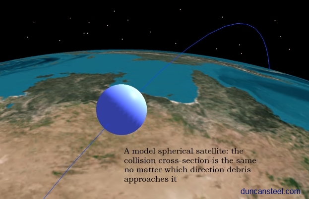
The collision probabilities derived above are in units of per square metre per year, and are based on a model test satellite in each case having a spherical shape and a geometrical cross-section (and therefore collision cross-section) of one square metre. Of course, the actual objects in question do not have such a size and shape.

The two are shown in the graphic below (the source of which is here). The Briz-M booster might be modelled as being near-enough to spherical for present purposes, with a characteristic size (diameter) of almost five metres, and so a cross-sectional area of about 20 square metres.

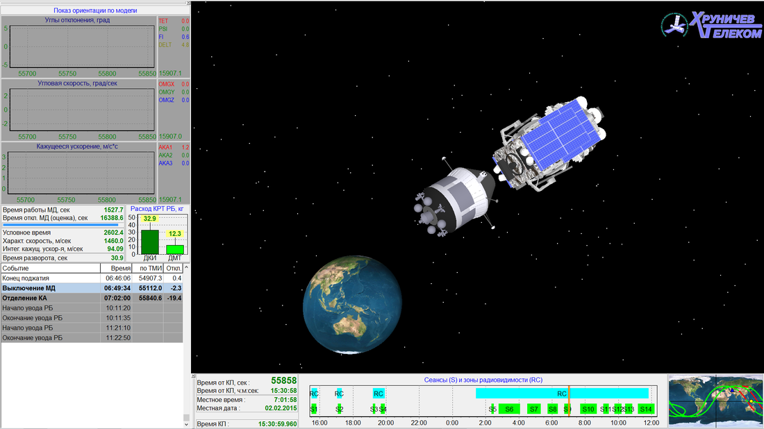
Graphic showing the Inmarsat-5F2 communications satellite (upper right) and the Briz-M rocket booster (centre). Courtesy Khrunichev.

The Inmarsat-5F2 satellite is much larger. Once its solar cells were deployed it attained a greatest linear dimension of 33.8 metres, and the thermal radiators and antennas that fold out from the main bus render linear dimensions of 8.08 metres. Looking at the satellite from orthogonal views its greatest cross-sectional area is therefore about 270 square metres, and its smallest about 65 square metres.

During its orbit around the Earth the satellite rotates its solar cells so as to keep these pointing towards the Sun, and the effect of this is to ‘average out’ the cross-section from the perspective of potential colliders such that again we might approximate its collision cross-section in terms of a sphere with a cross-sectional area of about 150 square metres, as a rough estimate.

Using that as a collision cross-section one derives a collision probability for the Inmarsat-5F2 satellite of about 5 × 10^-6 per year (i.e. 150 × 3.06 × 10^-8) and so a characteristic event rate of one collision per 200,000 years.

This value, however, is misleading: as noted earlier, most objects in the geostationary belt are moving in step, making it infeasible for them to collide with each other. One approach I could take here would be to sort through the 1,543 objects crossing the orbit of Inmarsat-5F2 and weed out those that are also truly geostationary or geosynchronous, making collisions with each other impossible in the present epoch, but it is sufficient to say simply that the true collision probability against other tracked objects is likely an order of magnitude less than the value calculated here (and so around 5 × 10^-7 per year, or a timescale of two million years).

Turning to the Briz-M rocket body, there is nothing to protect it from collisions with objects in the geostationary belt (or anywhere else). The collision probability for this object is therefore about 2.3 × 10^-8 per year (i.e. 20 × 1.15 × 10^-9) and the characteristic collision time is of order 40 million years.

In my first post here on orbital debris I discussed three different ways in which the ‘true’ collision probability could and would be higher than my calculations indicate, these ways being:
(i) The Satellite Situation Report and Two-Line Elements that are publicly-available do not include any CLASSIFIED orbits, these comprising almost 800 objects compared to the 16,167 in my listing used in these calculations;
(ii) Many of the tracked objects are larger than my model spherical satellite of cross-sectional area one square metre, so that the true collision cross-section for specific cases will be substantially larger than one square metre; and
(iii) The tracked objects are larger than about 10 cm in size, else they are not detectable with the ground-based optical and radar sensors employed by the U.S. military to keep tabs on anthropogenic orbiting objects, but fragmentation events such as remnant fuel explosions and hypervelocity collisions will produce many orbiting objects smaller than that 10 cm limit.

Taking each of these considerations in turn:
(i) There are certainly various CLASSIFIED payloads in geostationary orbit, and rocket bodies used to take them there also have GEO-crossing paths, but the effect of including these is unlikely to boost the derived net collision probability for objects in geostationary orbit by more than 50 per cent;
(ii) The communications satellites in GEO tend to be the largest objects in such orbits (unlike in LEO, where the International Space Station, the Hubble Space Telescope and various classified surveillance platforms dwarf most other satellites) so that the appropriate collision cross-sections to use are indeed the sizes of the communications satellites themselves, with areas dominated by solar cell arrays and typically being 100-300 square metres; and
(iii) There is very little small debris in orbits crossing the geostationary band, and so the enhancement in the collision probability due to sub-decimetre projectiles is small.

Overall my analysis leads to an expectation that the individual lifetimes of satellites in the geostationary band against catastrophic collisions with artificial space debris are of order millions to tens of millions of years.

 

Conclusions

I will now repeat what I have just written: the individual lifetimes of satellites in the geostationary band against catastrophic collisions with artificial space debris are of order millions to tens of millions of years.

If this conclusion is correct then, from the perspective of satellite protection and safety, there is no real need to boost defunct satellites into higher orbits, as is current practice. Indeed one might argue that to do so may have the effect of increasing the collision hazard: in any orbital manoeuvre there is a finite likelihood of something going wrong, perhaps with disastrous consequences. For example, re-igniting a rocket booster attached to a communications satellite, when that booster had been dormant for a decade or more since the satellite was placed in its desired station, might  lead to an explosion and thus the spreading of myriad pieces of debris around the geostationary belt with high relative velocities. It would be better to leave the satellite as it was, simply closing it down until future generations with better technical capabilities can clear it up.

If the debris impact timescale for geostationary orbits is indeed of order millions of years, the collisional impact risk for satellites in that high-altitude band is dominated by the flux of natural meteoroids. I will say nothing more on that subject here, and simply refer the reader to a recent report on the subject.

 

Dependence of the Orbital Debris Collision Hazard upon Inclination for Low-Earth Orbit Satellites

Duncan Steel
2015 April 28

 

Introduction

In my previous post concerning the orbital debris collision hazard for test satellites in low-Earth orbit (LEO) I used only two values of the inclination to the equator (30 and 98 degrees) as examples, that post being directed mainly towards elucidating how the collision probabilities vary with altitude. I wrote there that I would prepare another post that focusses upon the inclination-dependence: this is it.

The method and input orbital data for tracked objects used here are precisely the same as in that first post, and so I will not repeat what I presented there in that regard.

In Figure 1 below I show how the collision probability varies with the inclination of various test satellites (assumed spherical, cross-section one square metre) in circular orbits at differing altitudes in the LEO zone. The inclinations used go in ten degree steps from 0 to 180 degrees, except that three additional inclinations were inserted: 28.5 degrees (the geocentric latitude of Cape Canaveral), 45 degrees (near the latitude of the Baikonur launch site) and 98 degrees (the approximate inclination of satellites in sun-synchronous orbits in LEO).

Figure 1: Variation of the collision probability against the publicly-available orbits of tracked objects in geocentric orbit as a function of inclination for circular test satellite orbits at altitudes of
500, 700, 800, 900, 1000 and 1500 km.

Discussion

The following salient points can be understood from Figure 1:

1. Whilst all lines for any particular satellite altitude show peaks between 60 and 120 degrees, at higher inclinations (i.e. highly retrograde test orbits) the collision probabilities reduce. Given that the collision probability varies linearly with the relative velocity of potentially-colliding objects, and the fact that most of the tracked objects are in prograde orbits, this might not have been expected. The explanation for this feature (i.e. decreases in collision probability for highly retrograde orbits) is that if the orbital plane of the test satellite is close to the equator – whether prograde (i < 60 deg) or retrograde (i > 120 deg) – then that satellite spends much of each orbit at lower latitudes than the preponderance of tracked objects in near-polar orbits. This results in the overall collision probability being reduced.
2. The lines for test satellite altitudes 700, 800 and 900 km show broad maxima centred on inclination 80 degrees, and may be understood as being a result of the collision probability varying with the relative velocity of potentially-colliding objects: a satellite at such an inclination (say 80-100 degrees) has an elevated probability of colliding head-on with a piece of tracked debris (or indeed a functioning payload) that has a similar inclination but is travelling in the opposite direction. In addition, the collision between Cosmos 2251 (inclination 74 degrees) and Iridium 33 (inclination 86 degrees) at an altitude of about 789 km resulted in almost 2,000 items of tracked debris (and many smaller).
3. The highest collision probabilities are at altitudes of 700-900 km, consistent with my previous post.
4. Subsidiary maxima are seen at inclinations near 98 degrees at altitudes 800, 900, 1000 and 1500 km. These may be understood as being due to the larger populations of tracked items at or near this inclination, the possibility of being temporarily coplanar during cycles of precession of the nodes leading to increased collision probabilities. The reason for the larger populations near inclination 98 degrees include: (a) More satellites being inserted into orbits at altitudes above 800 km with such an inclination (i.e. sun-synchronous orbits); (b) The Chinese anti-satellite demonstration in 2007 January, when the weather satellite Fengyun-1C was destroyed in an orbit at altitude near 865 km and inclination 98.9 degrees, resulting in almost 3,000 items of tracked debris (and many more too small to be detected from the ground); (c) On 2015 February 03 the U.S. Defense Meteorological Satellite DMSP-F13, which had been launched in 1995, exploded in orbit at an altitude near 850 km and inclination 98.6 degrees, leaving hundreds of trackable fragments in nearby orbits.

 

Concluding remarks

There is one core point that I intended to make in this post: the probability of losing a functioning satellite due to a collision with orbital debris is not just a function of the satellite altitude: there is also a strong dependence on the orbital inclination (to the equator) that is chosen for the satellite. The information plotted in Figure 1 indicates that the collision probability at any altitude can vary by a factor of two or three across the full inclination range, with near-polar orbits being the most dangerous to occupy.

This post is just the second in a series in which I intend to describe and discuss various specific points regarding the orbital debris impact hazard for functioning satellites. Further posts will follow.

 

Assessment of the Orbital Debris Collision Hazard for Low-Earth Orbit Satellites

Duncan Steel
2015 April 26

Introduction

The fact that anthropogenic orbital debris (or ‘space junk’) poses a collision hazard to functioning satellites in geocentric orbits is well-known, although the level of the risk is not always recognised.

For example, there is often talk of the chance of communications satellites in geostationary orbit being struck by debris, disrupting global links and TV broadcasts, and from that notion stems the belief that once such satellites reach the end of their useful lives they should be boosted into higher orbits simply so as to obviate the risk of collisions with functioning payloads. This belief is false, as I will show in another post: at geostationary altitudes (circa 35,800 km above Earth’s surface) the probability of being struck by man-made debris, or other satellites, is tiny; and the impact risk is dominated by the hazard posed by natural meteoroids and interplanetary dust, which does not depend on the altitude.

On the other hand, in low-Earth orbit (LEO: altitudes below about 2,000 km) the population of debris and the relative velocities are such that the impact hazard posed by material we have launched into orbit is substantial, and too high to be ignored. The intent of the present paper is simply to illustrate the sorts of collision probabilities that exist in the present epoch.

The space debris problem has attracted the attention of the world’s space agencies, each of which has produced its own reports and recommendations over the past two or three decades, and also various national and international organizations such as the United Nations. There are too many reports that have been published to reference any but a few of them here. As an introduction I would just recommend to readers two substantial reports published in the last few years by US organisations: the RAND Corporation (Baiocchi & Welser, 2010) and the National Research Council (2011).

For my own part, my own work on the orbital debris problem began in 1988 when I established companies called Spaceguard Proprietary Limited (P/L) and SODA Software P/L (SODA meaning Spaceguard Orbital Debris Analysts) in South Australia. Much of the research I did then, having commercial applications, was not openly published. However, a few of the papers I did publish in following years, based on the software which I have used in deriving the results that appear in this post, are listed in the references below as Steel (1992a,b) and Dittberner et al. (1991).

The intent of the present post is not to give a final word on this matter, but rather to provide a primer for interested readers; I will be preparing further posts on the overall subject of orbital debris and the hazard it poses to present and planned satellites.

Input orbital data

In this analysis I have used all the objects available in the Satellite Situation Report (SSR), which is freely available from Space-Track.org (specifically, here). There were various inconsistencies that I identified in the SSR by comparison with the Two-Line Elements (TLEs: available from here). The SSR and TLE datasets used were the most recent available as at 2015 April 09.

My dataset compiled as above contained 40,586 objects, about 60 per cent of which have departed geocentric orbit: some of those have been sent on Earth-escaping paths (e.g. interplanetary probes) but the majority of the objects that are no longer in orbit are those which have re-entered the atmosphere. A total of 16,167 objects were found to have usable orbits for present purposes (i.e. determining collision probabilities with test/strawman satellite orbits).

Apart from that 16,167 there are about 800 objects still in geocentric orbit but listed in the publicly-available SSR as having “NO ELEMENTS AVAILABLE”. In general these are CLASSIFIED orbits: that is, they are Defence- or intelligence agency-related objects of the United States and its allies (including here launches by the United Kingdom, Germany, Israel and Japan, for example). That is, these are payloads, rocket bodies and debris associated with CLASSIFIED launches. Based on 800 being about five per cent of 16,167, one might imagine that the overall collision probability derived from the 16,167 orbits that are available might be about five per cent lower than the value which would result if all orbits were available for analysis; however, personal knowledge indicates that the CLASSIFIED launches include a disproportionate number of surveillance satellites placed into LEO, and many of these are high-mass and capable of producing a large amount of debris on fragmentation. In view of this I would anticipate that the net collision probability derived using the available 16,167 orbits is likely to be about 25 to 50 per cent lower than that which would result if the approximately 800 tracked CLASSIFIED orbits were also available for use here.

Apart from that consideration, of course the objects/orbits available are restricted to those which are large enough to be tracked using ground-based optical and radar sensors. For LEO this leads to a size limitation of about 10 cm (i.e. the size of a baseball, or a large orange) although the precise limit is dependent on several unknown factors separately for optical and radar detections. The fact is that several dozens of catastrophic on-orbit fragmentation events have occurred, and following such events only a minor fraction of the resultant debris items are detectable, those below 10 cm in size being expected to follow broadly similar orbits to the original object but not be trackable. It is believed that the number of debris items larger than 1 cm in size in LEO is above 100,000 and may well be substantially greater than that. Since a 1 cm object striking a functioning satellite at a speed of around 10 km/sec would be anticipated to cause calamitous damage, the net collision probability derived from only the 16,167 large tracked objects very much represents a lower bound for the overall debris impact risk. The real hazard is likely at least ten times higher.

For my own early assessment of the importance of smaller (untracked) fragments, please see Steel (1992a).

Method

The technique used to derive the collision probabilities between orbiting objects is that developed by Kessler (1981) and also described by Steel & Baggaley (1985). In the context of collisions between objects in heliocentric orbits (e.g. impacts of asteroids or comets on planets) the utility and possible limitations of Kessler’s method has been investigated by various researchers, for example Milani et al. (1990).

In the present instance I have used this method to derive collision probabilities between objects in geocentric orbits. Those orbits are described in terms of the semi-major axis (a), eccentricity (e) and inclination (i, referred to the equatorial plane) of each. Rather than a and e it is often simpler to provide input in terms of the perigee and apogee altitudes for all objects, and convert those into the geocentric perigee and apogee distances, and thence semi-major axes and eccentricities, for each object. In this report all altitudes are referred to the Earth equatorial radius of 6,378.137 km.

Kessler’s method involves a numerical integration of the collision probability values across all small volumes of space around the Earth which both orbiting objects can access. These small volumes or cells have dimensions defined in the software, and in these computations I have used radial steps of one kilometre and (geocentric) latitudinal steps of one degree. It is found that the results obtained for the collision probability asymptotically approach a constant value (for pairs of test orbits) as the fineness of these steps in radial distance and latitude are decreased, and the above adopted values render an acceptable trade-off between precision and computer execution time.

An essential assumption inherent in Kessler’s method is that the argument of perigee (AOP) and the longitude of the ascending node (LAN) are random, so that all AOP and LAN values have equal probabilities of occurrence. For objects in geocentric orbits that do not have controlled parameters (e.g. station-keeping) this will be the case, with the AOP and LAN values cycling quite rapidly. For the sake of interest and understanding I will make available some example movies here, demonstrating how the orbits of objects disperse upon fragmentation due to differential gravitational perturbations caused by the Earth’s non-sphericity.

The 3D view below introduces a set of modelled fragments of a satellite, originally in a circular orbit at altitude 900 km and with inclination 60 degrees, which disintegrates for some reason with the fragments having speeds relative to the original object (which was moving at close to 7.4 km/sec in orbit) of up to 0.8 km/sec. Enhanced orbital speeds render apogee altitudes up to 5,000 km; reduced orbital speeds drop the perigee, but any with perigee altitude below 200 km would soon re-enter due to atmospheric drag. I have assumed (for simplicity) that all fragments start off in the same orbital plane, but these soon spread due to differential precession rates. This graphic indicates the fragment positions about half-an-hour after the disintegration:

A movie is available here (27.8 MB) showing how these fragments disperse over the next eight hours. The 2D map that follows below indicates the spread of paths attained in just eight hours in terms of the sub-satellite/fragment tracks across the Earth’s surface, with a movie (4.45 MB) again being available for download from here.

The following 3D view shows how much the orbits have spread over the next 45 days, with a movie being available here (25.3 MB) which illustrates how quickly and widely this dispersal occurs.

It was mentioned above that Kessler’s method requires an assumption that both the AOP and the LAN of the two orbiting objects under consideration are random. Clearly this is not the case for, say, a satellite in a sun-synchronous polar orbit; however, the relative values of the AOP and LAN from one object (the satellite of interest, perhaps in such a controlled orbit) referred to the others (the debris in uncontrolled orbits) will be random, making the method a viable means for deriving collision probabilities.

 

Collision cross-sections

Unlike in encounters between interplanetary objects and the planets, no gravitational focussing is applicable in the case of these low-mass objects in geocentric orbit, and so only the geometrical cross-sections are of import.

For present purposes I have assumed that the test satellite is of spherical shape, so that the collision cross-section is the same no matter which direction the debris approaches it. This is shown schematically in the graphic below.

Because I wish to derive a collision probability per square metre per year, I model this spherical satellite to have a cross-sectional area of one square metre, which implies a radius of 56.4 centimetres.

Using this geometrical cross-section of one square metre as being the collision cross-section against each of the 16,167 tracked objects enables an overall collision probability to be derived, but again the value arrived at will be substantially lower than the true value because in reality the collision cross-section will be enhanced by the finite sizes of the colliding objects. That is, in effect I am assuming the potentially-colliding objects to have infinitesimally-small sizes, whereas in fact many of them are very substantial in size and indeed much bigger than this small model test satellite; consider the sizes of the Hubble Space Telescope or the International Space Station, for example.

To give a numerical example, consider a cylindrical rocket body two metres in diameter (and perhaps ten metres long) that happens to pass the spherical test satellite with its long axis aligned with its relative motion vector. If that long axis passes anywhere within one metre of the surface of the spherical test satellite then there will be a collision. This renders a minimum ‘miss’ distance of 1.564 metres, and so an enhancement of the collision cross-section by a factor of (1.564/0.564)² = 7.69. Given that the rocket body is far longer than it is wide, as it tumbles through space whilst moving along its orbit about Earth we should anticipate that its collision cross-section against the model spherical test satellite is substantially higher than this factor of 7.69, and will in fact be perhaps 20 or 30 times higher than the collision cross-section I am using here (i.e. simply the geometrical cross-section of the sphere). On the other hand, many of the tracked objects in the SSR are indeed much smaller than this model spherical test satellite, consisting of shards from exploded rocket bodies, an astronaut’s glove, a mislaid wrench, circuit boards, and so on. Overall the effect of the finite sizes of tracked objects might be to increase the collision probability for a small object (the one-square-metre sphere considered here) by a factor of two or three. In later analyses I will be attempting to assess this effect more accurately than this guesstimate of two or three used in the present post.

Results

For the present post I have restricted my analysis to test satellite orbits in two inclinations only: 30 degrees and 98 degrees. The former is typical for many LEO satellites (launches due eastwards attain inclinations equal to the geocentric latitude of the launch site, and Cape Canaveral is at 28.5 degrees latitude), whilst the latter is the approximate inclination required for a sun-synchronous polar orbit. In a future post I will examine how the collision probabilities vary with inclination for LEO satellites.

In Figure 1 below I show the collision probabilities obtained for test (spherical) satellites in circular orbits at different altitudes. All 16,167 tracked objects (as described earlier) are included in the calculations, but only limited numbers will have orbits crossing each test satellite altitude, and thus contribute to the overall collision probability. For example, for the test satellite orbits at altitude 800 km (the peaks of the plots in Figure 1) there were 4,535 tracked objects in all that might collide with those test satellites; the other 11,632 do not cross that 800 km altitude.

Figure 1: Total collision probability with test satellites in
circular orbits and with inclination 30 degrees (solid line)
and 98 degrees (dashed line).

An immediate question that might come to mind from a perusal of Figure 1 is this: why is the overall collision probability at all altitudes higher at inclination 98 degrees than at 30 degrees? The simple answer is that to first order the individual collision probabilities vary linearly with the collision speed, and the collision speeds are higher for high-inclination objects. Obviously this pushes up the overall collision probability, and also the likelihood of severe damage (due to the higher impact speed). Retrograde satellites and debris are disproportionately dangerous!

In Figure 2 I have plotted the collision probabilities for twenty test satellite orbits all with perigee altitude 300 km but apogees at heights between 300 km (i.e. a circular orbit) and 1,200 km (i.e. the highest eccentricity test orbit). A comparison of Figure 1 and Figure 2 indicates that the collision probabilities are reduced by a factor of about 2 in the latter. Why? The basic reason is that with reduced perigee altitudes the test satellites spend substantial time in each orbit lower down, where the population of tracked objects (debris etc.) is lower and this reduces the overall collision probability values, despite the fact that test satellite orbits with larger eccentricities (larger range between perigee and apogee) will cross the orbits of greater numbers of tracked orbiting items.

Figure 2: As Figure 1 but for non-circular test satellite orbits.
For each the perigee altitude is 300 km, with apogee altitudes as plotted along the x-axis.

In Figure 3 (below) the test satellites’ perigee altitude has been pushed up to 500 km, and this increases the net collision probability calculations by a small factor (compare Figures 2 and 3). Again one asks: why? The answer is that now the test orbits entail the satellites spending less time far from the densest region of tracked objects at altitudes between 700 and 900 km (cf. Figure 1).

Figure 3: As Figure 2 but perigee altitude 500 km.

In Figure 4 (below) the test orbit perigee has been increased to altitude 800 km. Now the net collision probability values are increased again from Figure 3, reaching comparable values to those presented in Figure 1. Of course the test orbits with perigee equal to apogee and equal to 800 km in Figure 4 are identical to those in Figure 1.

Figure 4: As Figure 2 but perigee altitude 800 km.

 

Discussion

The maximum values for net collision probabilities derived here are close to 1.4 x 10^-5 /m²/year, for orbits around 800 km altitude and high inclination. Previously it has been argued that the ‘real’ orbital debris collision probability would be substantially higher than the value calculated in this way for the tracked catalogue of objects in orbit, the enhancement appropriate being of the following order:

1. Higher by 25-50 per cent due to CLASSIFIED objects properly needing to be included in the assessment;
2. Higher by a factor of two or three due to the finite sizes of tracked objects compared to the one-square-metre spherical test satellite considered here; and
3. Higher by a factor of perhaps a hundred due to the large population of orbiting debris produced by fragmentation events that is smaller than the (approximately) 10 cm size limit for tracking from the ground by optical or radar means but nevertheless large enough to cause catastrophic damage to a functioning satellite in a hypervelocity impact.

If these enhancement factors are of the correct order, then the collision probability attains a value of around 5 x 10^-3 /m²/year, implying a lifetime of about 200 years against such collisions with orbital debris. This indicates that there is cause for concern: insert 200 satellites into such orbits and you should expect to lose about one per year initially, but then the loss rate would escalate because the debris from the satellites that have been smashed will then pose a much higher collision risk to the remaining satellites occupying the same orbits (in terms of a, e, i). This ‘self-collisional’ aspect of the debris collision hazard I highlighted in the early 1990s (Steel, 1992a), and I will be re-examining it in future posts.

 

Acknowledgements

I would like to thank Dr T.S. Kelso at the Analytical Graphics, Inc. (AGI) Center for Space Standards and Innovation in Colorado Springs for his assistance and advice on the contents and veracity of the Satellite Situation Report and Two-Line Elements files. I also thank AGI for the free use of the wonderful STK application, with which I produced the various graphics and movies that form part of this post.

 

References

Baiocchi, D. & Welser, W., ‘Confronting Space Debris’, RAND Corporation, Santa Monica, California, Report MG-1042-DARPA (2010).

Dittberner, G., J. Elder & D. Steel, ‘Orbital Debris Damage Estimates Using Coupled Pre- and Post-Impact Calculations’, 29th Aerospace Sciences Meeting of the American Institute of Aeronautics and Astronautics, Reno, Nevada; paper AIAA 91-0302 (1991). 

Kessler, D. J. ‘Derivation of the collision probability between orbiting objects: The lifetimes of Jupiter’s outer moons,’ Icarus, volume 48, pp.39-48 (1981).

Milani, A., M. Carpino & F. Marzari, ‘Statistics of Close Approaches between Asteroids and Planets: Project SPACEGUARD,’ Icarus, volume 88, pp.292-335 (1990).

National Research Council, ‘Limiting Future Collision Risk to Spacecraft: An Assessment of NASA’s Meteoroid and Orbital Debris Programs’, National Academies Press, Washington, D.C. (2011).

Steel, D. ‘The Space Station Will Eat Itself’, pp.271-276 in Hypervelocity Impacts in Space (edited by J.A.M. McDonnell), University of Kent, Canterbury, U.K. (1992a).

Steel, D. ‘Space Debris: Getting the Hazard into Perspective’, International Space Year in the Pacific Basin (edited by P.M.Bainum, G.L.May, M.Nagatomo, Y.Ohkami & Yang Jiachi), Advances in the Astronautical Sciences, volume 77, pp.243-254 (1992b).

Steel, D. I., & W. J. Baggaley 1985. ‘Collisions in the solar system-I. Impacts of Apollo-Amor-Aten asteroids upon the terrestrial planets. Monthly Notices of the Royal Astronomical Society, volume 212, pp. 817-836 (1985).