All posts by Duncan

Assessment of the Orbital Debris Collision Hazard for Low-Earth Orbit Satellites

Assessment of the Orbital Debris Collision Hazard for Low-Earth Orbit Satellites

Duncan Steel
2015 April 26

Introduction

The fact that anthropogenic orbital debris (or ‘space junk’) poses a collision hazard to functioning satellites in geocentric orbits is well-known, although the level of the risk is not always recognised.

For example, there is often talk of the chance of communications satellites in geostationary orbit being struck by debris, disrupting global links and TV broadcasts, and from that notion stems the belief that once such satellites reach the end of their useful lives they should be boosted into higher orbits simply so as to obviate the risk of collisions with functioning payloads. This belief is false, as I will show in another post: at geostationary altitudes (circa 35,800 km above Earth’s surface) the probability of being struck by man-made debris, or other satellites, is tiny; and the impact risk is dominated by the hazard posed by natural meteoroids and interplanetary dust, which does not depend on the altitude.

On the other hand, in low-Earth orbit (LEO: altitudes below about 2,000 km) the population of debris and the relative velocities are such that the impact hazard posed by material we have launched into orbit is substantial, and too high to be ignored. The intent of the present paper is simply to illustrate the sorts of collision probabilities that exist in the present epoch.

The space debris problem has attracted the attention of the world’s space agencies, each of which has produced its own reports and recommendations over the past two or three decades, and also various national and international organizations such as the United Nations. There are too many reports that have been published to reference any but a few of them here. As an introduction I would just recommend to readers two substantial reports published in the last few years by US organisations: the RAND Corporation (Baiocchi & Welser, 2010) and the National Research Council (2011).

For my own part, my own work on the orbital debris problem began in 1988 when I established companies called Spaceguard Proprietary Limited (P/L) and SODA Software P/L (SODA meaning Spaceguard Orbital Debris Analysts) in South Australia. Much of the research I did then, having commercial applications, was not openly published. However, a few of the papers I did publish in following years, based on the software which I have used in deriving the results that appear in this post, are listed in the references below as Steel (1992a,b) and Dittberner et al. (1991).

The intent of the present post is not to give a final word on this matter, but rather to provide a primer for interested readers; I will be preparing further posts on the overall subject of orbital debris and the hazard it poses to present and planned satellites.


Input orbital data

In this analysis I have used all the objects available in the Satellite Situation Report (SSR), which is freely available from Space-Track.org (specifically, here). There were various inconsistencies that I identified in the SSR by comparison with the Two-Line Elements (TLEs: available from here). The SSR and TLE datasets used were the most recent available as at 2015 April 09.

My dataset compiled as above contained 40,586 objects, about 60 per cent of which have departed geocentric orbit: some of those have been sent on Earth-escaping paths (e.g. interplanetary probes) but the majority of the objects that are no longer in orbit are those which have re-entered the atmosphere. A total of 16,167 objects were found to have usable orbits for present purposes (i.e. determining collision probabilities with test/strawman satellite orbits).

Apart from that 16,167 there are about 800 objects still in geocentric orbit but listed in the publicly-available SSR as having “NO ELEMENTS AVAILABLE”. In general these are CLASSIFIED orbits: that is, they are Defence- or intelligence agency-related objects of the United States and its allies (including here launches by the United Kingdom, Germany, Israel and Japan, for example). That is, these are payloads, rocket bodies and debris associated with CLASSIFIED launches. Based on 800 being about five per cent of 16,167, one might imagine that the overall collision probability derived from the 16,167 orbits that are available might be about five per cent lower than the value which would result if all orbits were available for analysis; however, personal knowledge indicates that the CLASSIFIED launches include a disproportionate number of surveillance satellites placed into LEO, and many of these are high-mass and capable of producing a large amount of debris on fragmentation. In view of this I would anticipate that the net collision probability derived using the available 16,167 orbits is likely to be about 25 to 50 per cent lower than that which would result if the approximately 800 tracked CLASSIFIED orbits were also available for use here.

Apart from that consideration, of course the objects/orbits available are restricted to those which are large enough to be tracked using ground-based optical and radar sensors. For LEO this leads to a size limitation of about 10 cm (i.e. the size of a baseball, or a large orange) although the precise limit is dependent on several unknown factors separately for optical and radar detections. The fact is that several dozens of catastrophic on-orbit fragmentation events have occurred, and following such events only a minor fraction of the resultant debris items are detectable, those below 10 cm in size being expected to follow broadly similar orbits to the original object but not be trackable. It is believed that the number of debris items larger than 1 cm in size in LEO is above 100,000 and may well be substantially greater than that. Since a 1 cm object striking a functioning satellite at a speed of around 10 km/sec would be anticipated to cause calamitous damage, the net collision probability derived from only the 16,167 large tracked objects very much represents a lower bound for the overall debris impact risk. The real hazard is likely at least ten times higher.

For my own early assessment of the importance of smaller (untracked) fragments, please see Steel (1992a).


Method

The technique used to derive the collision probabilities between orbiting objects is that developed by Kessler (1981) and also described by Steel & Baggaley (1985). In the context of collisions between objects in heliocentric orbits (e.g. impacts of asteroids or comets on planets) the utility and possible limitations of Kessler’s method has been investigated by various researchers, for example Milani et al. (1990).

In the present instance I have used this method to derive collision probabilities between objects in geocentric orbits. Those orbits are described in terms of the semi-major axis (a), eccentricity (e) and inclination (i, referred to the equatorial plane) of each. Rather than a and e it is often simpler to provide input in terms of the perigee and apogee altitudes for all objects, and convert those into the geocentric perigee and apogee distances, and thence semi-major axes and eccentricities, for each object. In this report all altitudes are referred to the Earth equatorial radius of 6,378.137 km.

Kessler’s method involves a numerical integration of the collision probability values across all small volumes of space around the Earth which both orbiting objects can access. These small volumes or cells have dimensions defined in the software, and in these computations I have used radial steps of one kilometre and (geocentric) latitudinal steps of one degree. It is found that the results obtained for the collision probability asymptotically approach a constant value (for pairs of test orbits) as the fineness of these steps in radial distance and latitude are decreased, and the above adopted values render an acceptable trade-off between precision and computer execution time.

An essential assumption inherent in Kessler’s method is that the argument of perigee (AOP) and the longitude of the ascending node (LAN) are random, so that all AOP and LAN values have equal probabilities of occurrence. For objects in geocentric orbits that do not have controlled parameters (e.g. station-keeping) this will be the case, with the AOP and LAN values cycling quite rapidly. For the sake of interest and understanding I will make available some example movies here, demonstrating how the orbits of objects disperse upon fragmentation due to differential gravitational perturbations caused by the Earth’s non-sphericity.

The 3D view below introduces a set of modelled fragments of a satellite, originally in a circular orbit at altitude 900 km and with inclination 60 degrees, which disintegrates for some reason with the fragments having speeds relative to the original object (which was moving at close to 7.4 km/sec in orbit) of up to 0.8 km/sec. Enhanced orbital speeds render apogee altitudes up to 5,000 km; reduced orbital speeds drop the perigee, but any with perigee altitude below 200 km would soon re-enter due to atmospheric drag. I have assumed (for simplicity) that all fragments start off in the same orbital plane, but these soon spread due to differential precession rates. This graphic indicates the fragment positions about half-an-hour after the disintegration:

M1

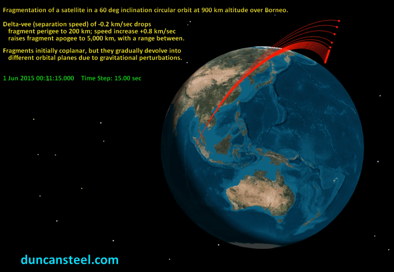
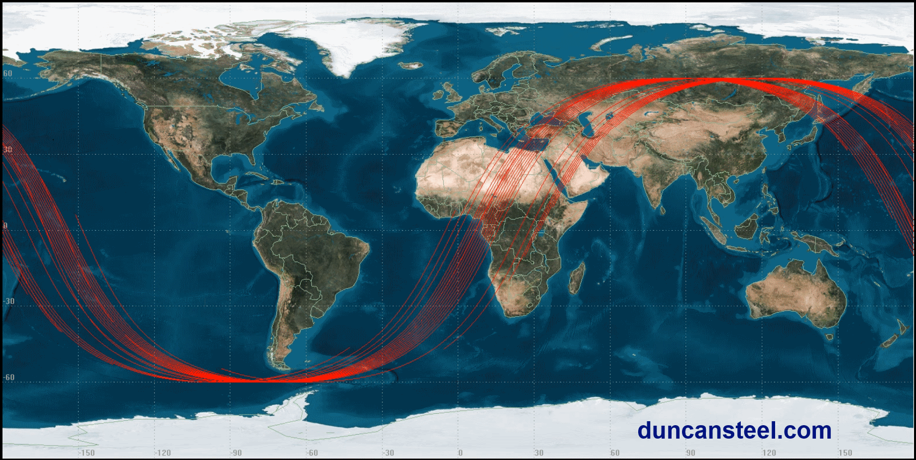
A movie is available here (27.8 MB) showing how these fragments disperse over the next eight hours. The 2D map that follows below indicates the spread of paths attained in just eight hours in terms of the sub-satellite/fragment tracks across the Earth’s surface, with a movie (4.45 MB) again being available for download from here.

M3

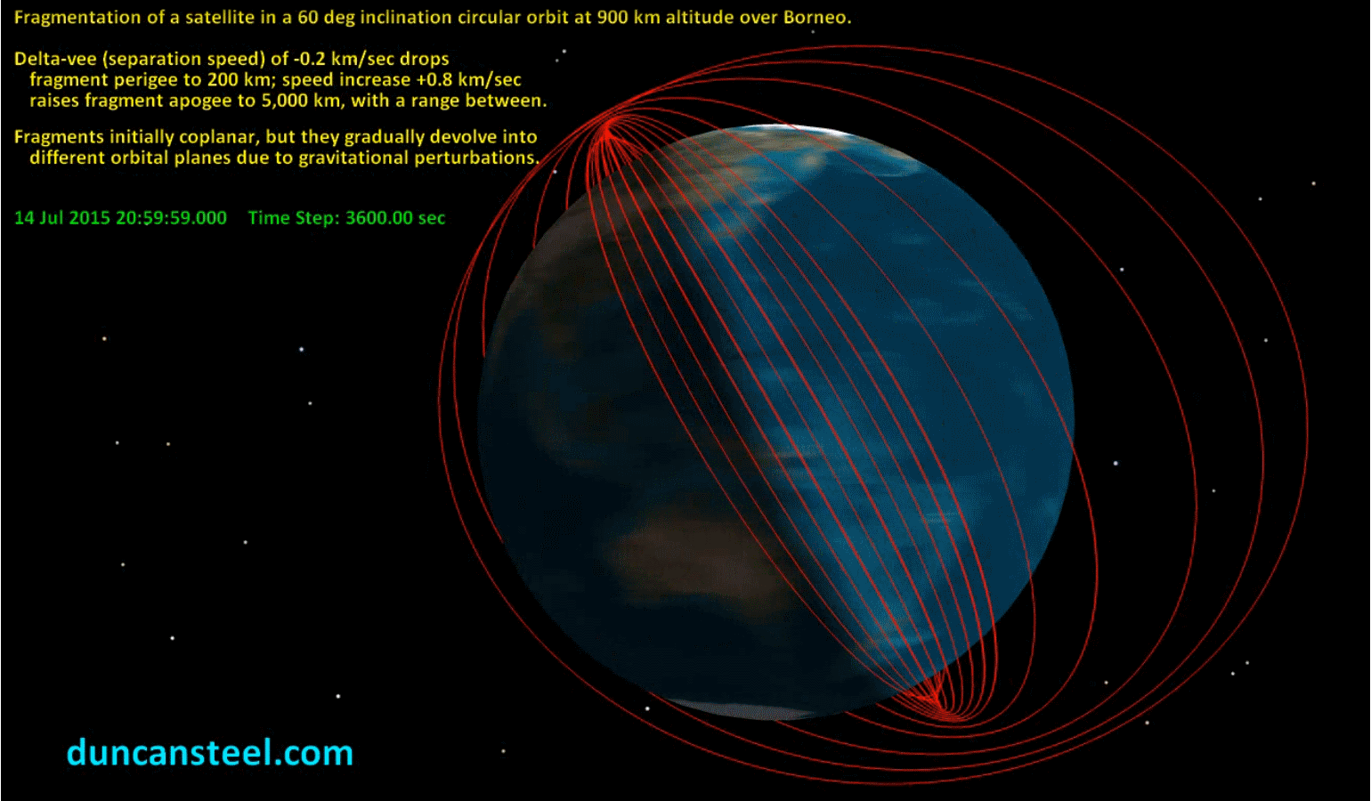
The following 3D view shows how much the orbits have spread over the next 45 days, with a movie being available here (25.3 MB) which illustrates how quickly and widely this dispersal occurs.

M2

It was mentioned above that Kessler’s method requires an assumption that both the AOP and the LAN of the two orbiting objects under consideration are random. Clearly this is not the case for, say, a satellite in a sun-synchronous polar orbit; however, the relative values of the AOP and LAN from one object (the satellite of interest, perhaps in such a controlled orbit) referred to the others (the debris in uncontrolled orbits) will be random, making the method a viable means for deriving collision probabilities.


Collision cross-sections

Unlike in encounters between interplanetary objects and the planets, no gravitational focussing is applicable in the case of these low-mass objects in geocentric orbit, and so only the geometrical cross-sections are of import.

For present purposes I have assumed that the test satellite is of spherical shape, so that the collision cross-section is the same no matter which direction the debris approaches it. This is shown schematically in the graphic below.

qr

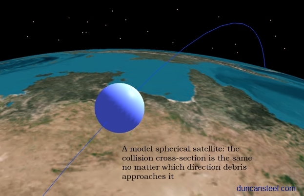
Because I wish to derive a collision probability per square metre per year, I model this spherical satellite to have a cross-sectional area of one square metre, which implies a radius of 56.4 centimetres.

Using this geometrical cross-section of one square metre as being the collision cross-section against each of the 16,167 tracked objects enables an overall collision probability to be derived, but again the value arrived at will be substantially lower than the true value because in reality the collision cross-section will be enhanced by the finite sizes of the colliding objects. That is, in effect I am assuming the potentially-colliding objects to have infinitesimally-small sizes, whereas in fact many of them are very substantial in size and indeed much bigger than this small model test satellite; consider the sizes of the Hubble Space Telescope or the International Space Station, for example.

To give a numerical example, consider a cylindrical rocket body two metres in diameter (and perhaps ten metres long) that happens to pass the spherical test satellite with its long axis aligned with its relative motion vector. If that long axis passes anywhere within one metre of the surface of the spherical test satellite then there will be a collision. This renders a minimum ‘miss’ distance of 1.564 metres, and so an enhancement of the collision cross-section by a factor of (1.564/0.564)2 = 7.69. Given that the rocket body is far longer than it is wide, as it tumbles through space whilst moving along its orbit about Earth we should anticipate that its collision cross-section against the model spherical test satellite is substantially higher than this factor of 7.69, and will in fact be perhaps 20 or 30 times higher than the collision cross-section I am using here (i.e. simply the geometrical cross-section of the sphere). On the other hand, many of the tracked objects in the SSR are indeed much smaller than this model spherical test satellite, consisting of shards from exploded rocket bodies, an astronaut’s glove, a mislaid wrench, circuit boards, and so on. Overall the effect of the finite sizes of tracked objects might be to increase the collision probability for a small object (the one-square-metre sphere considered here) by a factor of two or three. In later analyses I will be attempting to assess this effect more accurately than this guesstimate of two or three used in the present post.


Results

For the present post I have restricted my analysis to test satellite orbits in two inclinations only: 30 degrees and 98 degrees. The former is typical for many LEO satellites (launches due eastwards attain inclinations equal to the geocentric latitude of the launch site, and Cape Canaveral is at 28.5 degrees latitude), whilst the latter is the approximate inclination required for a sun-synchronous polar orbit. In a future post I will examine how the collision probabilities vary with inclination for LEO satellites.

In Figure 1 below I show the collision probabilities obtained for test (spherical) satellites in circular orbits at different altitudes. All 16,167 tracked objects (as described earlier) are included in the calculations, but only limited numbers will have orbits crossing each test satellite altitude, and thus contribute to the overall collision probability. For example, for the test satellite orbits at altitude 800 km (the peaks of the plots in Figure 1) there were 4,535 tracked objects in all that might collide with those test satellites; the other 11,632 do not cross that 800 km altitude.

Plot1

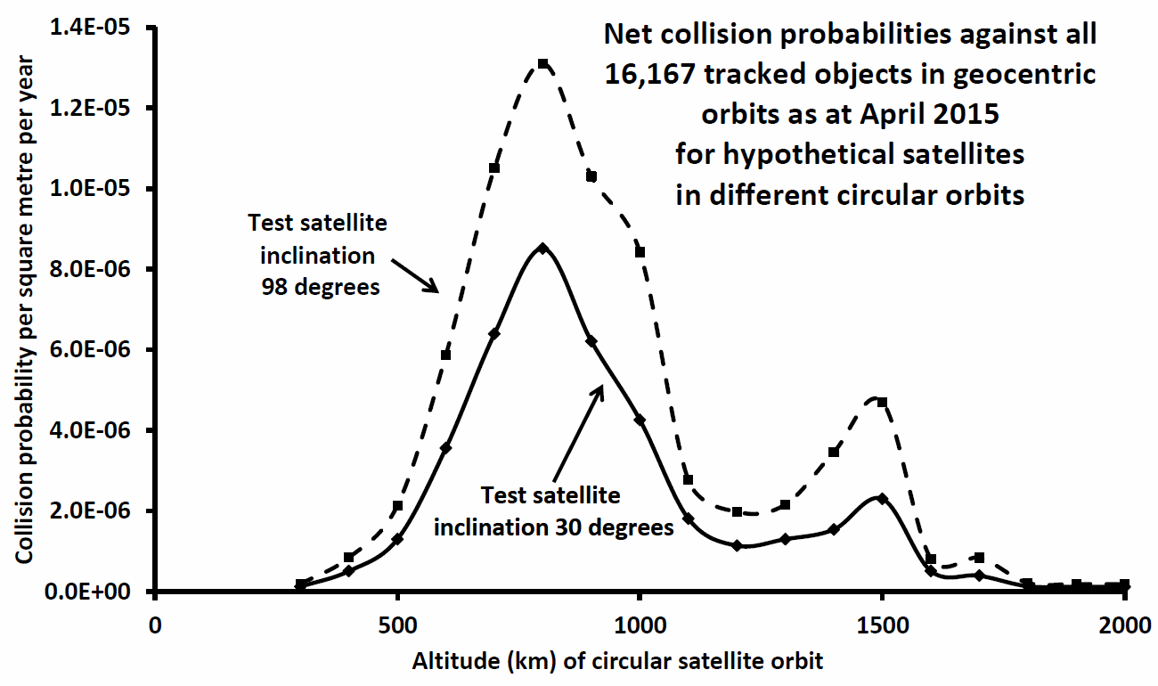
Figure 1: Total collision probability with test satellites in
circular orbits and with inclination 30 degrees (solid line)
and 98 degrees (dashed line).

An immediate question that might come to mind from a perusal of Figure 1 is this: why is the overall collision probability at all altitudes higher at inclination 98 degrees than at 30 degrees? The simple answer is that to first order the individual collision probabilities vary linearly with the collision speed, and the collision speeds are higher for high-inclination objects. Obviously this pushes up the overall collision probability, and also the likelihood of severe damage (due to the higher impact speed). Retrograde satellites and debris are disproportionately dangerous!

In Figure 2 I have plotted the collision probabilities for twenty test satellite orbits all with perigee altitude 300 km but apogees at heights between 300 km (i.e. a circular orbit) and 1,200 km (i.e. the highest eccentricity test orbit). A comparison of Figure 1 and Figure 2 indicates that the collision probabilities are reduced by a factor of about 2 in the latter. Why? The basic reason is that with reduced perigee altitudes the test satellites spend substantial time in each orbit lower down, where the population of tracked objects (debris etc.) is lower and this reduces the overall collision probability values, despite the fact that test satellite orbits with larger eccentricities (larger range between perigee and apogee) will cross the orbits of greater numbers of tracked orbiting items.

Plot2

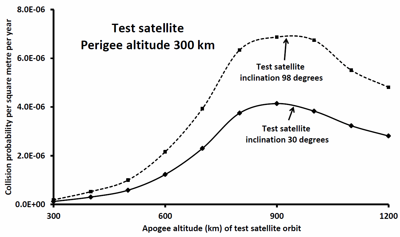
Figure 2: As Figure 1 but for non-circular test satellite orbits.
For each the perigee altitude is 300 km, with apogee altitudes as plotted along the x-axis.

In Figure 3 (below) the test satellites’ perigee altitude has been pushed up to 500 km, and this increases the net collision probability calculations by a small factor (compare Figures 2 and 3). Again one asks: why? The answer is that now the test orbits entail the satellites spending less time far from the densest region of tracked objects at altitudes between 700 and 900 km (cf. Figure 1).

Plot3

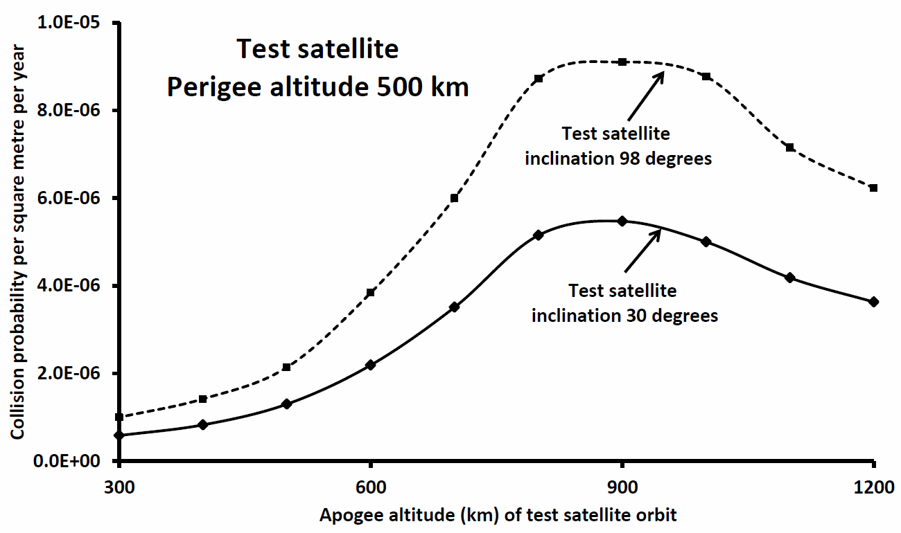
Figure 3: As Figure 2 but perigee altitude 500 km.

In Figure 4 (below) the test orbit perigee has been increased to altitude 800 km. Now the net collision probability values are increased again from Figure 3, reaching comparable values to those presented in Figure 1. Of course the test orbits with perigee equal to apogee and equal to 800 km in Figure 4 are identical to those in Figure 1.

Plot4

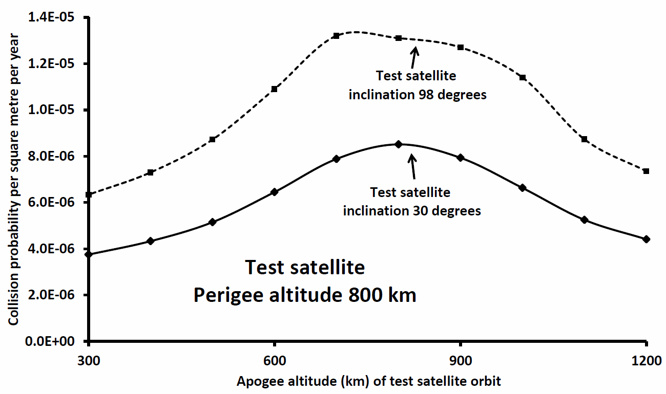
Figure 4: As Figure 2 but perigee altitude 800 km.


Discussion

The maximum values for net collision probabilities derived here are close to 1.4 x 10⁻⁵ /m2/year, for orbits around 800 km altitude and high inclination. Previously it has been argued that the ‘real’ orbital debris collision probability would be substantially higher than the value calculated in this way for the tracked catalogue of objects in orbit, the enhancement appropriate being of the following order:

  1. Higher by 25-50 per cent due to CLASSIFIED objects properly needing to be included in the assessment;
  2. Higher by a factor of two or three due to the finite sizes of tracked objects compared to the one-square-metre spherical test satellite considered here; and
  3. Higher by a factor of perhaps a hundred due to the large population of orbiting debris produced by fragmentation events that is smaller than the (approximately) 10 cm size limit for tracking from the ground by optical or radar means but nevertheless large enough to cause catastrophic damage to a functioning satellite in a hypervelocity impact.

If these enhancement factors are of the correct order, then the collision probability attains a value of around 5 x 10⁻³ /m2/year, implying a lifetime of about 200 years against such collisions with orbital debris. This indicates that there is cause for concern: insert 200 satellites into such orbits and you should expect to lose about one per year initially, but then the loss rate would escalate because the debris from the satellites that have been smashed will then pose a much higher collision risk to the remaining satellites occupying the same orbits (in terms of a, e, i). This ‘self-collisional’ aspect of the debris collision hazard I highlighted in the early 1990s (Steel, 1992a), and I will be re-examining it in future posts.


Acknowledgements

I would like to thank Dr T.S. Kelso at the Analytical Graphics, Inc. (AGI) Center for Space Standards and Innovation in Colorado Springs for his assistance and advice on the contents and veracity of the Satellite Situation Report and Two-Line Elements files. I also thank AGI for the free use of the wonderful STK application, with which I produced the various graphics and movies that form part of this post.


References

Baiocchi, D. & Welser, W., ‘Confronting Space Debris’, RAND Corporation, Santa Monica, California, Report MG-1042-DARPA (2010).

Dittberner, G., J. Elder & D. Steel, ‘Orbital Debris Damage Estimates Using Coupled Pre- and Post-Impact Calculations’, 29th Aerospace Sciences Meeting of the American Institute of Aeronautics and Astronautics, Reno, Nevada; paper AIAA 91-0302 (1991)

Kessler, D. J. ‘Derivation of the collision probability between orbiting objects: The lifetimes of Jupiter’s outer moons,’ Icarus, volume 48, pp.39-48 (1981).

Milani, A., M. Carpino & F. Marzari, ‘Statistics of Close Approaches between Asteroids and Planets: Project SPACEGUARD,’ Icarus, volume 88, pp.292-335 (1990).

National Research Council, ‘Limiting Future Collision Risk to Spacecraft: An Assessment of NASA’s Meteoroid and Orbital Debris Programs’, National Academies Press, Washington, D.C. (2011).

Steel, D. ‘The Space Station Will Eat Itself’, pp.271-276 in Hypervelocity Impacts in Space (edited by J.A.M. McDonnell), University of Kent, Canterbury, U.K. (1992a).

Steel, D. ‘Space Debris: Getting the Hazard into Perspective’, International Space Year in the Pacific Basin (edited by P.M.Bainum, G.L.May, M.Nagatomo, Y.Ohkami & Yang Jiachi), Advances in the Astronautical Sciences, volume 77, pp.243-254 (1992b).

Steel, D. I., & W. J. Baggaley 1985. ‘Collisions in the solar system-I. Impacts of Apollo-Amor-Aten asteroids upon the terrestrial planets. Monthly Notices of the Royal Astronomical Society, volume 212, pp. 817-836 (1985).


Autopilot Flight Path BFO Error Analysis

 Autopilot Flight Path BFO Error Analysis

Yap Fook Fah
2015 March 24

(Updated 2015 April 20 to make the BTO and BFO Calculator available online: see reference [4] added at the very end.) 

A downloadable PDF of this report (867 kB) is available here.

  1. Background

This report presents a Burst Frequency Offset (BFO) data error analysis of the end-game flight path of MH370 constrained by certain autopilot flight modes. The analysis is broadly similar in approach to that outlined in the ATSB reports [1, 2], but from which crucial quantitative results are not available for independent study.

Recall that the current search area is mainly defined by a compromise between two methods of analysis: “Constrained Autopilot Dynamics” (CAD), and “Data Error Optimisation” (DEO), as outlined in [1].

The CAD method assumes that the flight, at least after 18:40 UTC, was on some autopilot mode, and its range is limited by the amount of remaining fuel and aircraft performance. The ATSB report did not specify the time and location of the final major turn to the south. Further, the report did not provide details on how the generated paths were scored according to their “statistical consistency with the measured BFO and BTO values” [2].

In contrast, the DEO method does not take into account the flight mode, but simply seeks to rank a set of curved flight paths according to the deviation of the calculated BFO for each candidate flight path from the recorded values at the arc crossings after 18:40 UTC.

One problem is that the results from the two analyses are not quite consistent with each other. In particular, the DEO results imply that paths ending in the southern half of the CAD probability curve should be ranked much lower and be given less weight. In consequence, this has led to a compromise in the definition of the search area: “Area of interest on 0019 arc covers 80% of probable paths from the two analyses at 0011 …” [1]. This has the effect of shifting the search region further north than if only the CAD results were considered (see Figure 1 below).

Yap Fig 1

Figure 1: Defining the search area (from reference [1]).


  1. Objective

The objective of the present report is to reconstruct the end-game flight path BFO data error analysis with autopilot constraints, so as to obtain quantitative results for further evaluation and comparison with other types of analysis.


  1. Methodology 
  • A set of flight paths is generated starting from different locations on the 19:41 arc, each location being reachable from the last known radar position at 18:22 with the aircraft flying at feasible speeds.
  • Each path is a rhumb line (or loxodrome) corresponding to a constant true track autopilot mode. The exercise is repeated assuming great circle paths (geodesics). The WGS84 model for the shape of the Earth is used.
  • Each path is assumed to be flown at constant altitude. The exercise is repeated with an assumed rate of descent starting at 00:11 UTC (2014 March 08) that minimizes the BFO error.
  • All paths cross the arcs at the recorded times, and therefore match the Burst Timing Offset (BTO) values exactly.
  • The ground speed is allowed to vary. The speed profile is derived using a cubic polynomial function fitted over the five points at 19:41, 20:41, 21;41, 22:41 and 00:11. Integration of the speed over time gives the correct distance values at the arc crossings.
  • A BFO fixed frequency bias of 150.26 Hz is used [3].
  • The BFO values at the five arc crossings are calculated and compared to the recorded BFO values. The root-mean-square (RMS) error for each path is then calculated.


  1. Results

Figures 2 through 5 are based on the paths southwards after 19:41 being rhumb lines (i.e. loxodromes), whereas Figures 6 and 7 are based on the modelled paths being great circles (i.e. geodesics).

Figure 2 shows, as a function of the assumed aircraft latitude at 19:41, (a) the variation of the minimum RMS BFO error; and (b) the latitude attained at 00:19, based on the rate of descent at 00:19 being optimized (i.e. the BFO value at that time being fitted).

Figure 3 is similar to Figure 2, but represents the azimuth of the derived rhumb line path from the position at 19:41.

Figures 4 and 5 are similar to Figures 2 and 3 except that they result from assuming no descent (a level flight) at 00:11.

Figure 6, for a great circle path as described above, is similar to Figure 2 in that the minimum RMS BFO error and the latitude attained at 00:19 is depicted, based on the rate of descent at 00:19 being optimized.

Figure 7 is similar to Figure 3: the minimum RMS BFO error and the latitude attained at 00:19 is depicted, based on no descent (a level flight) at 00:11.

Obviously there are no graphs/figures for constant azimuths in the case of these great circle (geodesic) paths because such paths have constantly-changing azimuths.

Yap Fig 2

Figure 2: Rhumb line paths with optimized rate of descent at 00:11
indicating possible latitudes attained at 00:19.
(Note: R.O.C. means ‘Rate Of Climb’, which has negative values for a descent.)

 Yap Fig 3

Figure 3: Rhumb line paths with optimized rate of descent at 00:11
indicating possible azimuths of such paths.


Yap Fig 4


Figure 4: Rhumb line paths based on a constant altitude/no descent
at 00:11, 
indicating possible latitudes attained at 00:19.

 Yap Fig 5

Figure 5: Rhumb line paths based on a constant altitude/no descent
at 00:11, 
indicating possible azimuths of such paths.

 Yap Fig 6

Figure 6: Geodesic paths based on an optimized rate of descent at 00:11
indicating possible latitudes attained at 00:19.


Yap Fig 7

Figure 7: Geodesic paths, based on a constant altitude/no descent
at 00:11, indicating possible latitudes attained at 00:19.

 The most important points from the results shown in Figures 2 through 7 may be summarized as in Table 1:

Yap Table 1

Table 1: Summary of results

Two interesting observations may be made concerning the optimum rhumb line path:

  • If that path is extended back towards the north from 19:41, it passes close to waypoints ANOKO and IGOGU, as shown in Figure 8 below.
  • Examining that path as it moves southwards on azimuth 186.6T, it is found to pass close to waypoint ISBIX, as shown in Figure 9 below.

A Skyvector plot of the overall optimum rhumb line path is available from here.

Yap Fig 8

Figure 8: Propagating the optimum rhumb line flight path back northwards from 19:41.

Yap Fig 9

Figure 9: The optimum rhumb line flight path passes close to waypoint ISBIX.


  1. Conclusions

The calculations presented here are based on a BFO error analysis assuming both (i) rhumb line/loxodrome; and (ii) great circle/geodesic paths, but without assuming any particular location and time of the final major turn. These calculations lead to a prediction of a set of likely flight paths and locations of the aircraft at 00:19, which have been ranked according to the RMS BFO error.

It is estimated that the path with the smallest RMS BFO error has a constant azimuth (i.e. is a rhumb line) of 186.6 degrees True; an end-point location (i.e. position at 00:19) that is near (-37.5, 89.0);  and a course that passes close to the three waypoints IGOGU, ANOKO and ISBIX.

The sensitivity of the RMS BFO error to changes in track and end-point location from the optimum solution appears to be quite low; consequently any location from latitude -34.5 to latitude -40.5 lying along the 7th ping arc cannot be ruled out based on BFO error analysis alone.  The search zone could possibly be reduced further by considering other factors such as aircraft performance. That is, this analysis has been based on DEO alone (allowing curved paths), with no CAD considerations involved (except for allowable paths being limited to rhumb lines or geodesics).

The analysis discussed herein could be further refined by considering the sensitivity to BTO errors, the fixed frequency bias utilized in the BFO analysis, and the rate of climb along the path (which has been assumed here to be zero – level flight – through until at least 00:11). This is beyond the scope of the current work, but preliminary studies suggest that the general conclusions reported here still hold.

Finally, it is to be emphasized that the analysis and results presented here are based on the standard interpretation of the BTO and BFO data. Assuming that the BTO and BFO data are reliable, the following Table 2 summarizes a compelling argument for a flight by an autopilot mode to the Southern Indian Ocean (SIO).

Yap Table 2

Table 2: Summary of arguments for an autopilot flight
to the Southern Indian Ocean.

  1. Acknowledgements

I thank all members of the Independent Group (IG) for the active discussion and comments which have greatly helped me to understand much of the information that supports this analysis.


  1. References

[1] ATSB (Australian Transport Safety Bureau) report (08 October 2014): Flight Path Analysis Update.

[2] ATSB (Australian Transport Safety Bureau) report (26 June 2014; updated 18 August 2014): MH370 – Definition of Underwater Search Areas

[3] Richard Godfrey (19 December 2014): MH370 Flight Path Model version 13.1

[4] The BTO and BFO Calculator is available for download from here.

Deducing the Mid-Flight Speed of MH370

Deducing the Mid-Flight Speed of MH370

Brian Anderson 
2015 March 20

(Document prepared 26 December 2014)


  1. Introduction 

Contact was lost with the crew of Malaysia Airlines flight MH370 at about 17:20 UTC on 7th March 2014. Despite extensive searches no trace has yet been found. Later in March 2014 the Inmarsat company released limited information regarding communications between MH370 and the Inmarsat-3F1 satellite, illustrating two hypothetical tracks southwards into the Indian Ocean, one at a constant speed of 400 knots, and one at 450 knots. A redacted version of the Inmarsat communication log was released at the end of May 2014. Specifically, the Burst Timing Offset (BTO) data released in the log file enabled a more accurate determination of the locations the so-called ‘ping rings’, and the distances of these rings from the sub-satellite position.

At about this time many other people, Inmarsat and the ATSB among them, made attempts to illustrate possible flight paths, choosing assumed speeds in order to intercept the ping rings at the appropriate times. It was very clear that the speed assumptions were not much more than guesses, and most flight paths required changes of aircraft heading at each ping ring in order to fit against the known travel times between those rings. Figures 1 and 2 illustrate some of these guesses; many other examples could be given.

BAfig1

Figure 1: An early example of putative paths to the Southern Indian Ocean using assumed speeds of 450 knots (yellow) and 400 knots (red).

BAfig2

Figure 2: An example of early priority search regions (since recognized to be incorrect). The intent in showing this example is to illustrate how various path models used changes of directions at the ping ring locations, which is obviously non-physical.  

The purpose of this paper is to show that it is possible to deduce the speed of MH370 in the mid-flight phase (specifically between about 19:41 and 20:41 UTC) using minimal data from the Inmarsat logs. The resulting value for the speed agrees well with the known speed of the aircraft soon after it had reached cruise altitude following take-off and before its turn back at 17:21 UTC near waypoint IGARI.

This hypothesis regarding how the aircraft speed might be deduced was first proposed in May 2014 (see below). The calculation was refined and updated progressively with new data over the following few weeks. This paper is a consolidation of a number of blog contributions during that period, in order to present the hypothesis in a concise fashion.


  1. Initial observations

Before any BTO data were available, certain information was presented to a briefing of the Chinese families of MH370 passengers, at the Lido Hotel in Beijing, on about 28 April 2014. One of the slides presented became known as the ‘Fuzzy Chart of Elevation Angles’. This chart is shown below as Figure 3. Interestingly, the elevation angles (i.e. the apparent angular elevation of the satellite as seen from the aircraft; or, 90 degrees minus the zenith angle of the satellite as viewed from the aircraft) must have been derived from calculations based on the BTO data, but at this point no BTO data had been released publicly.

BAfig3

Figure 3: The Fuzzy Chart of Elevation Angles
derived from Inmarsat BTO values.

While this chart shows only a few data points it became the basis for various attempts at reverse-engineering the BTO data and thence the ping rings, and specifically the radii for these rings. At this time the Inmarsat definition for the BTO could be interpreted a number of different ways, and vigorous debate ensued amongst outside observers to determine the correct interpretation. Different interpretations resulted in radius variations of up to 50 NM (nautical miles).

In observing the elevation data points it is clear that the aircraft travelled away from the satellite immediately after take-off, then reversed its track and was coming closer to the satellite at least until about 19:40 UTC, then began moving away from the satellite again.

The reversal between 19:40 and 20:40 (approach to the satellite switching to recession)  is interesting in that there is clearly an instant between these two times when the aircraft was nearest to the satellite, and the elevation angle was therefore at a maximum. One can infer from this simple observation that at the point of closest approach the aircraft was therefore flying tangentially to the satellite.

From the fuzzy chart alone one could estimate the time of the closest approach at perhaps 12 minutes after 19:40. Work done by members of the Independent Group (IG) enabled the ping ring radii* at 19:40 and 20:40 to be estimated. An estimate of the elevation angle at the time of closest approach also enabled the calculation of the tangential radius. This was first suggested in a comment posted on May 16.

*In reality the ping rings or arcs are defined by equal ranges (as derived from the BTO values when they became available) from the satellite to the aircraft. Even if the aircraft were flying at a constant altitude (referred to either the WGS84 ellipsoid or Mean Sea Level, MSL) the ping rings would not truly be circular, because the Earth is not spherical. Regardless, using the term ‘radius’ to denote the sizes of the ping rings appears sensible, and for present purposes – estimating the aircraft’s speed averaged over an hour – the ping rings are indeed assumed to be arcs of circles.


  1. Initial calculations

Armed with just three pieces of derived information – the estimated time of closest approach, and the radii of the 19:40 and 20:40 ping rings – it is possible to derive an estimate for the speed of the aircraft between these times (posted May 17; see also further comments posted on May 18 and May 20). One substantive assumption is necessary: that the aircraft was travelling in a straight line between these time, or nearly so. A slightly curved track would result in a greater distance being travelled, and hence a slightly greater speed being appropriate (than the lesser speed obtained from the method described here). Of course it is also necessary to assume a more-or-less constant speed between these times/between these ping rings.

Recognising that the geometry can be represented by two right-angled triangles, having a common/shared side (see Figure 4), planar geometry allows a solution for the length of the bases for these triangles to be determined, and hence the speed of the aircraft.

BAfig4

Figure 4: Geometry enabling the average aircraft speed between the
circa. 19:40 and circa. 20:20 pings to be estimated. 

Let:

r1 = radius for the 19:40 ping ring

r2 = radius for the 20:40 ping ring

r0 = radius at the tangential point

t1 = time interval from 19:40 to the tangential point occurrence (12 minutes)

t2 = time interval from the tangential point occurrence to 20:40 (48 minutes)

d1 = distance travelled from 19:40 to the tangential point

d2 = distance travelled from the tangential point through to 20:40

v = the average speed of the aircraft between 19:40 and 20:40

Then:

d12 = r12 – r02

d22 = r22 – r02

d1 = (t1/60) * v

d2 = (t2/60) * v

(The division by 60 converts the time interval from minutes to fractions of an hour.)

Note that the radius to the tangential point (r0) does not need to be known since it can be eliminated from the two equations above.

Rearranging:   v = √(r22r12) / ((t2 /60)2 – (t1/60)2)

The initial values for r1 and r2 derived from the Fuzzy Chart were 1815 and 1852 NM respectively. Using these values and solving for v renders the aircraft speed as 476 knots.

This speed is significantly greater than most of the published guesses that were prevalent at the time.

A planar geometry solution to what is of course a spherical geometry situation is likely to result in a only a rough approximation, but the results were significant, and sufficiently encouraging to persist with the methodology while seeking accurate BTO data, an accurate satellite ephemeris, and solving the triangles using spherical geometry; as follows.


  1. Better input data, more accuracy

A redacted Inmarsat communications log was released publicly towards the end of May 2014, providing a set of BTO values (delay times). By that time, ten weeks after loss of MH370, the correct interpretation of the Inmarsat BTO calculation had been established by Mike Exner [1], a member of the IG. This and the BTO data enabled a more accurate determination of the line-of-sight (LOS) range from the satellite to the aircraft, more precise timing for the ping ring intercepts, and an accurate calculation of the elevation angles first presented in the Fuzzy Chart (and then reverse-engineered to provide the satellite-aircraft ranges used earlier, as in section 3 above).

With new and reliable satellite ephemeris data it was also possible to perform accurate calculations for the ping ring radii from the correctly-timed sub-satellite position.

The speed deduction was improved by using these data and also a more-accurate estimation of the time of occurrence of the tangential point, using the minimum LOS L-Band transmission delay [1].

Figure 5 shows the calculated L-Band transmission delays for BTO data after 18:28 UTC.

BAfig5

Figure 5: The L-Band time delays for the aircraft-satellite link as a function of time during the flight of MH370.

 A third-order polynomial curve is fitted to the data points in Figure 5, leading to a solution:

Y = -0.0038x3 + 0.4433x2 – 13.116x + 237.91

Differentiating this equation so as to determine the time of the minimum LOS range between the satellite and the aircraft:

dy/dx = -0.0114x2 + 0.8866x – 13.116

When dy/dx = 0 one obtains

x = 19.870 (or 57.9015)

Converting this to a time, this yields an interval of 11.20 minutes after 19:41 UTC.

Note that it is by no means certain that the BTO for 18:28 UTC should fit conveniently on the smooth curve fitted to the LOS range delay. This might imply that the aircraft track from that time was more-or less a straight line, but there is no information to suggest that this is so.

In order to lessen the significance of that data point (at 18:28) a new nominal point was introduced at time 19:01.  A LOS range was determined for this point by fitting to the LOS range curve. It was hypothesised that turns which the aircraft may have made at around 18:28 to establish a track south would be well completed by 19:01, and hence this point ought to sit on the more-or-less straight track extending through 19:41 and 20:41. A nominal BTO figure was reverse-engineered for this nominal point.

With the new data it is also possible to calculate more accurate ping ring radii for the new precisely-determined times, 19:41:03 and 20:41:05 (as opposed to the approximate 19:40 and 20:40 read off the Fuzzy Chart), coupled with the accurate satellite ephemeris. Radii of 1757.25 and 1796.56 NM were used to solve once again the two right-angled triangles, but this time using spherical geometry.

Using the same nomenclature:

Let:

r1 = radius for the 19:41 ping ring, expressed in radians

r2 = radius for the 20:41 ping ring, expressed in radians

r0 = radius at the tangential point, expressed in radians

t1 = time after 19:41 that the tangential point occurs (11.2 minutes)

t2 = time after the tangential point to 20:41 (48.8 minutes)

D = Great Circle distance travelled between 19:41 and 20:41

v = average speed of the aircraft between 19:41 and 20:41

Then:               cos(r1) = cos(r0) * cos(D * t1/(t1 + t2))

and                  cos(r2) = cos(r0) * cos(D * t2/(t1 + t2))

v = D/(t1 + t2)

The ground speed calculated by this method is now 494 knots.

The wind speed and direction for a potential southern track over this segment is about 21 knots from 65 degrees True [2]. Using this wind information, and the above ground speed of 494 knots on a track azimuth of 186 degrees, one can calculate the KTAS (True Air Speed, Knots) for the aircraft as being approximately 484 knots.

The fact that the KTAS matches the aircraft speed during cruise towards IGARI on the early portion of the flight adds a degree of confidence in this result, and provides a valuable basis for track and path estimates for later in the flight.

The astute may note that there is still an approximation (or implicit assumption) made in performing this calculation. This is due to the fact that the satellite is not stationary (although it is nearly so at about 19:41, having reached the apogee in its near-circular, 1.7-degree inclined orbit). This means that the apices of the right-angled triangles formed by the two ping radii and the tangent are not exactly coincidental. The error introduced by this assumption/approximation is small, and within the likely error margin from the estimated wind vectors for that location, and possible variations in ping ring radii from known BTO truncation and jitter. The range of sub-satellite positions is illustrated in Figure 6.

BAfig6

Figure 6: The movement of the sub-satellite position during the flight of MH370. In effect the method used in this paper assumes that the satellite remains in the same position between 19:41 and 20:41 UTC; the error caused by this necessary assumption is small.
Source: the above is Figure 8 in the paper published in the Journal of Navigation by Ashton et al. (2014).

  1. Speed limits and observations

Since the speed obtained from this calculation is dependent upon the precise estimation of the time of the closest approach to the satellite (i.e. the tangent position), it is sensible to explore the possible limits of speed that might result from variations in this estimate.

It is sufficient to establish a maximum speed from published Boeing 777 performance data. A Mach number M=0.85 might be regarded as an upper limit, and this results in a KTAS of about 510 knots, depending on altitude and ambient temperature assumptions.

A special case exists when the tangent position occurs precisely at 19:41 (i.e. on the ping ring). In this case there is only one right-angled triangle to be solved. The ground speed derived for this case is 392 knots. For this occurrence to be true the LOS range from the satellite would have to exhibit its minimum precisely at 19:41. Examination of the numbers for LOS range, the BTO and the elevation angles suggest that this is not the case, and that the tangent point occurs after 19:41 (and well before 20:41).

One can therefore conclude that speeds less than 400 knots, or greater than 510 knots, are not plausible. It might also be reasonable to conclude that the aircraft was in fact close to the normally expected cruise speed, and also close to the normally expected cruise altitude of 35,000 ft.

In terms of aiding the overall understanding of the flight and therefore the speed of the aircraft it would be useful to know what autopilot Cost Index (CI) was programmed into the Flight Management Computer (FMC) for this flight. The IG has appealed several times for the CI used/programmed to be made available, but so far Malaysia Airlines has declined to do so. With such information in hand the IG would be able to refine its understanding of the constraints which can be placed on the flight: for example, knowing the CI would enable the likely speed(s) to be narrowed down, and knowing the fuel load the feasible flying range would be better defined and thus knowledge of the most-likely end-point refined.

References:

[1] Exner, M.L.: Deriving Net L-Band Propagation Delay and Range from BTO Values, 2014 May 28.

[2] Source for wind information is here.

Acknowledgements:

I thank everyone who assisted in discussions of this idea. This includes members of the IG, but also the various people who helped with their own comments and suggestions when I first proposed the concept.

This paper is available for download as a PDF (680 kB) from here.